SMOKE provides two ways of processing mobile sources. (Recall that by “mobile sources” in SMOKE we mean on-road mobile sources.) The first approach is to compute mobile emissions values prior to running SMOKE and provide them to SMOKE as input; we call this the precomputed-emissions approach. The second approach is to provide SMOKE with VMT data, meteorology data, and MOBILE6 inputs, and have SMOKE compute the mobile emissions based on these data; this is called the VMT approach. These approaches are not mutually exclusive, so it is possible to provide both precomputed emissions and VMT data to SMOKE and have the system compute only some of the emissions using MOBILE6. Both processing approaches can produce criteria, particulate, and toxics emissions results.
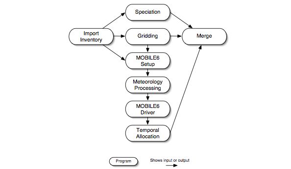
The precomputed-emissions approach is quite similar to the processing method for area sources. In fact, Figure 2.8, “Base case area-source processing steps”, Figure 2.9, “Future- or past-year growth and optional control area-processing steps”, and Figure 2.10, “Alternative future- or past-year growth and control area-processing steps” from Section 2.8.2, “Area-source processing” show exactly the processing steps needed for processing mobile sources using SMOKE and the precomputed-emissions approach. As in base-case processing for area sources, emissions in the inventory file are subdivided to hourly emissions during temporal allocation, assigned chemical speciation factors during speciation, and assigned spatial allocation factors during gridding. The merge step combines the hourly emissions, speciation matrix, and gridding matrix to create model-ready emissions. For future- or past-year processing, the growth and controls step is added to create the growth and control matrices, while the grow inventory step converts the inventory from the base year to a future or past year. The control matrix can be optionally used in the merge step to apply control factors to the future- or past-year emissions. Note that, unlike the VMT approach, in the precomputed-emissions approach SMOKE will not model the variations in emissions caused by temperature, humidity, or other meteorological settings.
The VMT approach is much different from the precomputed-emissions approach. Figure 2.13, “Base case mobile VMT approach processing steps” summarizes the VMT approach. First, VMT data (both link and county-total) by road class and vehicle type are input to SMOKE. The chemical speciation step computes the chemical speciation factors for each county, road class, vehicle type, emissions process (e.g., exhaust start, exhaust running, evaporative, hot soak, diurnal), and pollutant and stores the necessary factors for this transformation. The gridding step allocates the link sources to grid cells and uses spatial surrogates to allocate county-total emissions to grid cells, storing the factors needed for these allocations. The gridding step also creates “ungridding” factors which are used to create county-based meteorology data in the meteorology processing step.
Before the meteorology processing, a MOBILE6 setup program is run which uses inventory and grid information to create inputs for the meteorology processing step. The meteorology processing step uses information from the MOBILE6 setup step and the “ungridding” factors created by the gridding step to compute county-specific hourly temperatures, barometric pressures, and humidity values, which are fed to the MOBILE6.2 driver to compute hour-specific emission factors. The temporal allocation step combines the VMT and emission factors and makes other temporal adjustments to obtain hour-specific emissions for each emissions process. Finally, the merge step combines the hourly emissions, spatial allocation factors, and chemical speciation factors to calculate model-ready emissions.
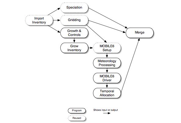
In addition to base-case processing, the VMT approach can also be used for future- or past-year processing and for control cases. Figure 2.14, “Future- or past-year growth and control mobile-source processing steps” summarizes the steps needed for such processing. In addition to the steps in Figure 2.13, “Base case mobile VMT approach processing steps”, the grow inventory step is used to grow the VMT data to the future year. In the MOBILE6 driver step, the system can use MOBILE6.2 entries that contain settings for the future/past year, as well as control settings such as those related to inspection and maintenance programs.
In sections later in this chapter, we describe the SMOKE programs that are needed for each of the processing steps just described for mobile sources, and additional details about what activities are accomplished during each step. These sections are:
- Section 2.9, “Inventory import”
- Section 2.10, “Temporal processing”
- Section 2.11, “Chemical speciation processing”
- Section 2.12, “Spatial processing”
- Section 2.13, “Growth processing”
- Section 2.14, “Control processing”
- Section 2.16, “On-road mobile-source processing with MOBILE6”
- Section 2.18, “Creating model-ready emissions”
- Section 2.19, “Quality assurance”
Processing mobile sources involves a number of concepts that are unique to mobile sources. These include the link optional source characteristic, a special approach for on-road mobile SCCs, special codes used for road classes and facility types, road types in MOBILE6, SMOKE and MOBILE6 vehicle types, emissions processes, MOBILE6 emission factors, reference counties, and the use of gridded meteorology data. The following subsections explain these topics in more detail.
Mobile sources have an optional source characteristic known as link sources. For SMOKE purposes, links are straight road segments within a county and are defined by starting and ending lat-lon or UTM coordinates. Curved roads must be broken into several straight segments to approximate the curved shape. A Geographical Information Systems (GIS) program and a travel demand model are typically used to perform link-source input preparation; these activities are not integrated into SMOKE. The link coordinates must be provided as input data to SMOKE if you want to use link data. This approach provides the advantage of improved spatial allocation for model-ready emissions, because the VMT and therefore emissions are assigned directly to grid cells using the coordinates, rather than relying on spatial surrogates.
In SMOKE, links are identified by 15-character alphanumeric link IDs, which must be unique for each combination of FIPS code and SCC. SMOKE contains its own line-grid intersection routine to allocate the link emissions into each grid cell. The links are allocated to the cells by the fraction of length of each segment within each grid cell; this allocation is performed by the Grdmat program, which assumes that VMT or emissions data are uniformly distributed over the link.
SMOKE handles SCCs differently for on-road mobile sources compared with all other source categories. SMOKE programs assume that on-road mobile SCCs have the following form:
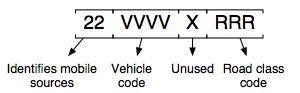
The Smkinven program populates SMOKE’s internal fields for vehicle type (vehicle code) and road type by extracting them from the SCC and converting the 3-digit road class to the 2-digit road type (using the mapping provided in the MCODES file). During cross-referencing for any mobile-source processing step, SMOKE builds internal SCCs of the form:
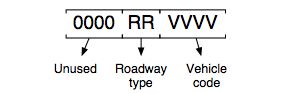
These internal SCCs are created by SMOKE for both the inventory file and the cross-reference file. Therefore, any information included in the unused “X” portion of the inventory SCC will be ignored during the cross-referencing. If you refer to the on-road mobile cross-referencing hierarchies provided with each program that uses cross-referencing in Chapter 6, SMOKE Core Programs, the vehicle type and road type are a part of the hierarchy, but the inventory SCC code is not. The internal SCCs are used so that the correct hierarchy can be used (in which the vehicle type is a more specific descriptor). See Section 2.3.5, “Source Classification Codes” for a description of the “left to right” hierarchy of the parts of an SCC.
In some cases, SMOKE errors and warnings that appear when processing on-road mobile sources will contain the internal SCC instead of the source’s inventory SCC. The information provided in this section can help you determine which source is actually a concern.
Although the “X” portion of the inventory SCC is not used as part of the cross-referencing assignments in SMOKE, it is important that any SCC that appears in the cross-reference file also appear in the inventory in exactly the same way. This is because SMOKE filters the cross-reference files before using them by comparing the SCC in the cross-reference file to the complete list of SCCs in the inventory. This comparison considers the “X” portion of the SCC, and if the SCC that you want to use is in the cross-reference with a different “X” than what is in the inventory, the cross-reference record will be dropped and will not be applied to the sources.
The Aerometric Information Retrieval System (AIRS) AMS road class code is the same as the last three digits in the 10-digit SCC expected by SMOKE. Within SMOKE, the road class is stored as the two-digit combination of the area type code and facility type code. Descriptions of the road classes and their associated numeric codes are as given in Table 2.2, “AMS road class and corresponding area and facility type”.
Table 2.2. AMS road class and corresponding area and facility type
| Name | AIRS AMS road class code | Area type code | Facility type code |
|---|---|---|---|
| Rural Interstate | 110 | 0 | 1 |
| Rural Principal Arterial | 130 | 0 | 2 |
| Rural Minor Arterial | 150 | 0 | 6 |
| Rural Major Collector | 170 | 0 | 7 |
| Rural Minor Collector | 190 | 0 | 8 |
| Rural Local | 210 | 0 | 9 |
| Urban Interstate | 230 | 1 | 1 |
| Urban Freeway | 250 | 1 | 2 |
| Urban Principal Arterial | 270 | 1 | 4 |
| Urban Minor Arterial | 290 | 1 | 6 |
| Urban Collector | 310 | 1 | 7 |
| Urban Local | 330 | 1 | 9 |
MOBILE6 can model five different road types: freeway, arterial, local, freeway ramp, and none (used for emission processes that are not road dependent, such as exhaust start and hot soak). Table 2.3, “Road class and corresponding MOBILE6 road type” indicates how the 12 road classes listed in Table 2.2, “AMS road class and corresponding area and facility type” are mapped to the five MOBILE6 types. Local roads can be modeled using either (1) MOBILE6’s local road type, which applies an average speed of 12.9 mph, or (2) the arterial road type and the average speed given in the mobile-source inventory.
Table 2.3. Road class and corresponding MOBILE6 road type
| Name | MOBILE6 Road Type |
|---|---|
| Rural Interstate | freeway, freeway ramp |
| Rural Principal Arterial | arterial |
| Rural Minor Arterial | arterial |
| Rural Major Collector | arterial |
| Rural Minor Collector | arterial |
| Rural Local | local or arterial |
| Urban Interstate | freeway, freeway ramp |
| Urban Freeway | freeway, freeway ramp |
| Urban Principal Arterial | arterial |
| Urban Minor Arterial | arterial |
| Urban Collector | arterial |
| Urban Local | local or arterial |
Note that SMOKE assumes that a portion of the VMT data supplied for interstates and freeways are attributable to freeway ramps. Therefore, SMOKE computes a composite emission factor from the freeway and freeway ramp emission factors from MOBILE6 and maps the composite to the interstates and freeways.
The vehicle types used in SMOKE’s on-road mobile source processing are described in Table 2.4, “Vehicle type codes and descriptions”. The codes (e.g., 0100) should be used in the cross-reference files.
Table 2.4. Vehicle type codes and descriptions
| Code | Description |
|---|---|
| 0100 | LDGV: Light Duty Gasoline Vehicles |
| 0102 | LDGT1: Light Duty Gasoline Trucks 1 |
| 0104 | LDGT2: Light Duty Gasoline Trucks 2 |
| 0107 | HDGV: Heavy Duty Gasoline Vehicles |
| 3000 | LDDV: Light Duty Diesel Vehicles |
| 3006 | LDDT: Light Duty Diesel Trucks |
| 3007 | HDDV: Heavy Duty Diesel Vehicles |
| 0108 | MC: Motorcycles |
MOBILE6 produces emission factors for a total of 28 vehicle types. For SMOKE to assign these emission factors to the mobile sources, the emission factors must be aggregated to the eight vehicle types listed in Table 2.4, “Vehicle type codes and descriptions”. To perform this aggregation, the emission factors for each MOBILE6 vehicle type are weighted by the percentage of VMT assigned to that vehicle type (using the default MOBILE6 values or values assigned by the VMT FRACTIONS command), then summed over the vehicle types to create emission factors for the eight SMOKE vehicle types. Table 2.5, “MOBILE6 vehicle type and corresponding SMOKE vehicle type” lists the MOBILE6 vehicle types and the corresponding SMOKE vehicle types.
Table 2.5. MOBILE6 vehicle type and corresponding SMOKE vehicle type
| MOBILE6 Vehicle Types | SMOKE Vehicle Type |
|---|---|
| LDGV: Light Duty Gasoline Vehicles (Passenger Cars) | LDGV |
| LDGT1: Light Duty Gasoline Trucks 1 (0-6,000 lbs. GVWR, 0-3,750 lbs. LVW) | LDGT1 |
| LDGT2: Light Duty Gasoline Trucks 2 (0-6,000 lbs. GVWR, 3,751-5,750 lbs. LVW) | LDGT1 |
| LDGT3: Light Duty Gasoline Trucks 3 (6,001-8,500 lbs. GVWR, 0-5,750 lbs. ALVW) | LDGT2 |
| LDGT4: Light Duty Gasoline Trucks 4 (6,001-8,500 lbs. GVWR, >5,751 lbs. ALVW) | LDGT2 |
| HDGV2b: Class 2b Heavy Duty Gasoline Vehicles (8,501-10,000 lbs. GVWR) | HDGV |
| HDGV3: Class 3 Heavy Duty Gasoline Vehicles (10,001-14,000 lbs. GVWR) | HDGV |
| HDGV4: Class 4 Heavy Duty Gasoline Vehicles (14,001-16,000 lbs. GVWR) | HDGV |
| HDGV5: Class 5 Heavy Duty Gasoline Vehicles (16,001-19,500 lbs. GVWR) | HDGV |
| HDGV6: Class 6 Heavy Duty Gasoline Vehicles (19,501-26,000 lbs. GVWR) | HDGV |
| HDGV7: Class 7 Heavy Duty Gasoline Vehicles (26,001-33,000 lbs. GVWR) | HDGV |
| HDGV8a: Class 8a Heavy Duty Gasoline Vehicles (33,001-60,000 lbs. GVWR) | HDGV |
| HDGV8b: Class 8b Heavy Duty Gasoline Vehicles (>60,000 lbs. GVWR) | HDGV |
| HDGB: Gasoline Buses (School, Transit, and Urban) | HDGV |
| LDDV: Light Duty Diesel Vehicles (Passenger Cars) | LDDV |
| LDDT12: Light Duty Diesel Trucks 1 and 2 (0-6,000 lbs. GVWR) | LDDT |
| LDDT34: Light Duty Diesel Trucks 3 and 4 (6,001-8,500 lbs. GVWR) | LDDT |
| HDDV2b: Class 2b Heavy Duty Diesel Vehicles (8,501-10,000 lbs. GVWR) | HDDV |
| HDDV3: Class 3 Heavy Duty Diesel Vehicles (10,001-14,000 lbs. GVWR) | HDDV |
| HDDV4: Class 4 Heavy Duty Diesel Vehicles (14,001-16,000 lbs. GVWR) | HDDV |
| HDDV5: Class 5 Heavy Duty Diesel Vehicles (16,001-19,500 lbs. GVWR) | HDDV |
| HDDV6: Class 6 Heavy Duty Diesel Vehicles (19,501-26,000 lbs. GVWR) | HDDV |
| HDDV7: Class 7 Heavy Duty Diesel Vehicles (26,001-33,000 lbs. GVWR) | HDDV |
| HDDV8a: Class 8a Heavy Duty Diesel Vehicles (33,001-60,000 lbs. GVWR) | HDDV |
| HDDV8b: Class 8b Heavy Duty Diesel Vehicles (>60,000 lbs. GVWR) | HDDV |
| HDDBT: Diesel Transit and Urban Buses | HDDV |
| HDDBS: Diesel School Buses | HDDV |
| MC: Motorcycles (Gasoline) | MC |
SMOKE can use all of the emissions-forming processes modeled in the MOBILE6 model. These processes are the following.
-
EXR: exhaust running emissions
-
EXS: exhaust engine start emissions (trip start)
-
HOT: evaporative hot soak emissions (trip end)
-
DNL: evaporative diurnal emissions (heat rise)
-
RST: evaporative resting loss emissions (leaks and seepage)
-
EVR: evaporative running loss emissions
-
CRC: evaporative crankcase emissions (blow-by)
-
RFL: evaporative refueling emissions (fuel displacement and spillage)
-
BRK: particulate matter from brake component wear
-
TIR: particulate matter from tire wear
“Emission types” are the combinations arising from combining the above emission-forming processes with each of the pollutants output by MOBILE6, for example, EXR__NOX or EVR__TOG. Each emission type is associated with emission factors produced by the MOBILE6 emission factor model. SMOKE currently supports many process-and-pollutant combinations that are output by MOBILE6; the list below indicates which pollutants can be combined with each process. Note that the list below does not include the user-defined toxics pollutants generated by using the ADDITIONAL HAPS command in SMOKE. Note also that only one hydrocarbon output can be used at a time (e.g., either VOC or TOG [total organic gases] but not both). In the examples below, TOG could be replaced with any of the other hydrocarbon pollutants available from MOBILE6: total hydrocarbons (THC), non-methane hydrocarbons (NMHC), VOC, TOG, or non-methane organic gases (NMOG).
-
EXR: all pollutants except particulates from brake and tire wear
-
EXS: CO, NOX, TOG, BENZENE, MTBE, BUTADIENE, FORM, ACETALD, ACROLEIN
-
HOT: TOG, BENZENE, MTBE
-
DNL: TOG, BENZENE, MTBE
-
RST: TOG, BENZENE, MTBE
-
EVR: TOG, BENZENE, MTBE
-
CRC: TOG
-
RFL: TOG, BENZENE, MTBE
-
BRK: BRAKE25, BRAKEPMC
-
TIR: TIRE25, TIREPMC
Emission factors are created in SMOKE using MOBILE6, for a wide variety of emission processes and pollutants. Some of the MOBILE6 input commands implement control strategies (e.g., inspection and maintenance [I/M] programs, antitampering programs [ATPs], and reformulated gas [RFG]). Other MOBILE6 inputs define other factors contributing to the value of the emissions factors, such as vehicle registrations (which help define the mix of different vehicle types), fuel volatility parameters, speeds, and temperature. All of these different dependencies make mobile emissions processing more complex than other types of sources.
When running MOBILE6, each county in the mobile inventory is assigned a reference county using the MCREF file. All counties with the same reference county will use the same MOBILE6 input scenario. The MOBILE6 input scenario defines many aspects to be modeled, including I/M programs, ATPs, and fuel parameters.
For a single county, SMOKE duplicates the MOBILE6 input scenario for all speeds in the inventory. It then inserts county-specific temperature, barometric pressure, and humidity data (see Section 2.8.4.8, “Use of gridded meteorology data”, replaces speed information, and runs MOBILE6. The hourly emission factors are then matched to the individual sources and stored.
SMOKE retains its performance benefits when processing mobile sources through the use of “ungridded” county-based meteorology data. SMOKE calculates averaged temperature, humidity, and barometric pressure data by averaging the individual data in the grid cells intersecting each county, weighted by the fraction of the VMT in that county intersecting those grid cells. The ungridding is implemented by building an “ungridding matrix”, MUMAT, which must be created by the Grdmat program.
Because the MOBILE6 emission factors used by SMOKE are significantly influenced by temperature and, to a lesser extent, humidity, the most desirable approach from an accuracy standpoint is to model mobile emissions using gridded, temporalized data from a meteorological model. However, to retain the performance benefits of source-based SMOKE processing, SMOKE has been designed to “ungrid” the meteorology data to get county-based data. For processing of all kinds, SMOKE expects data from one of the gridded, hourly meteorology files MET_CRO_2D or MET_CRO_3D. The MET_CRO_2D file is used for ground, 1.5-meter, or 10-meter temperature data. The MET_CRO_3D data file is used for ambient temperature, barometric pressure, and water vapor mixing ratio data. These data can be used to calculate absolute and relative humidity data needed for MOBILE6. For on-road mobile processing, the surface temperature from the MET_CRO_2D file is usually used along with the pressure and mixing ratio data from the MET_CRO_3D file; these files must be combined into a single file using the Metcombine utility (see Section 5.6, “Metcombine”).
MOBILE6 has the ability to use 24-hour temperature profiles, 24-hour relative humidity data, and daily barometric pressure data. SMOKE uses the gridded meteorology data to create these profiles for each county in the inventory. To save processing time, SMOKE can create spatially or temporally averaged 24-hour temperature and humidity profiles, resulting in fewer MOBILE6 runs.
-
Spatial averaging: For each reference county, SMOKE can either create separate temperature and humidity profiles for each inventory county, or it can create one profile by averaging data from all counties sharing the reference county. Note that all counties sharing the same reference county are usually within the same state, so this kind of spatial averaging would not result in averaging counties from different states.
-
Temporal averaging: Using this type of averaging, SMOKE can create a 24-hour temperature and humidity profile for each day of the episode (no averaging), or a temperature and humidity profile for each week or month in the episode. Finally, SMOKE can create one temperature and humidity profile for the entire episode, averaging over all days within the episode.
Options for spatial and temporal averaging of meteorology data are independent by county, and are set in the MVREF settings file.