The temporal allocation of emission inventory data always occurs after the inventory import processing previously described in Section 2.8, “Inventory import”. The Temporal program processes data for anthropogenic sources, while the Tmpbeis3 or Tmpbeis4 program allocates biogenic emissions. In this section, we focus on the temporal allocation of the anthropogenic inventories using Temporal. The biogenic processing is further described in Section 2.16, “Biogenic processing”.

The primary purpose of the Temporal program is to create an intermediate hourly emissions file (ATMP, MTMP, or PTMP). It also creates a supplementary intermediate file that indicates which monthly, weekly (day-of-week), and diurnal (hourly) profiles were assigned to each source (ATSUP, MTSUP, or PTSUP). Since the Temporal dynamically create names for the output files, two new environment variables [A|M|P]TMPNAME and [A|M|P]TSUPNAME are used to set the directory and file prefix for naming the output files [A|M|P]TMP and [A|M|P]TSUP. The files are named using the starting date of each time period.For example, if ATMPNAME is set to /data/ntmp.nctox., then the ATMP file for a given time period will be put in the data directory and named ntmp.nctox.[start date].ncf.

The temporal processing operation applies factors based on the source characteristics to the emissions data from the SMOKE inventory files. These factors can include monthly, weekly, and diurnal temporal profiles. The resulting emissions data vectors (not a matrix) contain hourly emissions for the inventory species. SMOKE assumes an hourly time step (Even though the time step is an input setting to SMOKE, it currently cannot be changed.). Most of the calculations are implemented as sparse-matrix algebra based upon temporal cross-references and profiles, augmented by the substitution of values from day- and hour-specific emissions data sets. For mobile sources, hourly emissions values also depend on meteorology (e.g., the temperature dependence of evaporative emissions).

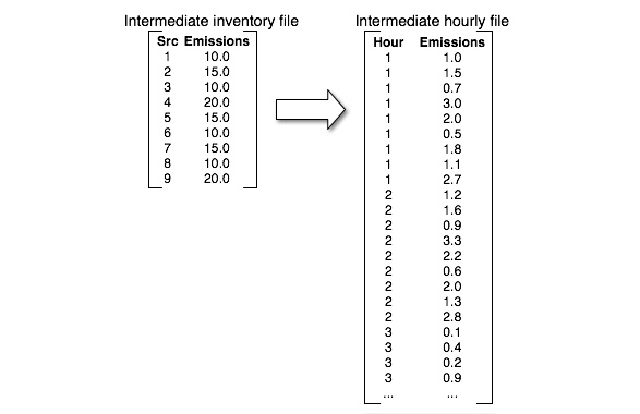
Figure 2.20, “Transformation of inventory data to hourly data” shows how data from the intermediate inventory are stored in the hourly file. The arrow represents the temporal processing steps which convert the annual, average-day, or day- and hour-specific data to hourly data. After the temporal processing, the hourly emissions are stored in the intermediate hourly file, by hour and source number. The emissions are stored in the same order as the sources in the sorted intermediate inventory file.

Temporal processing also addresses the following issues that need to be considered during emissions processing:

In the subsections below, we address each of these issues in the same order as the list above.