The paradigm for atmospheric emissions models prior to SMOKE was a network of pipes and filters. This means that at any given stage in the processing, an emissions file includes self-contained records describing each source and all of the attributes acquired from previous processing stages. Each processing stage acts as a filter that inputs a stream of these fully-defined records, combines it with data from one or more support files, and produces a new stream of these records. Redundant data are passed down the pipe at the cost of extra I/O, storage, data processing, and program complexity. Using this method, all processing is performed one record at a time, without necessarily a structure or order to the records.

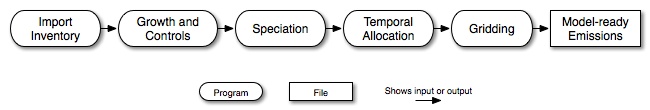
This old paradigm came about as a way to avoid repeatedly searching through data files for needed information, which would be very inefficient. It is admirably suited to older computer architectures with very small available memories and tape-only storage, but is not suitable for current desktop machines or high-performance computers. SMOKE developers demonstrated this when the Emissions Preprocessor System (EPS) 2.0 was run on a Cray Y-MP. It ran four times slower on the Cray machine (a much faster computer) than on a desktop 150 MHz DEC Alphastation 3000/300. This paradigm also fostered a serial approach to the emissions processing steps, as shown in Figure 2.3, “Serial approach to emissions processing”.

The new paradigm implemented in SMOKE came about from analyses indicating that emissions computations should be quite adaptable to high-performance computing if the paradigm were appropriately changed. For each SMOKE processing category (i.e., area, biogenic, mobile, and point sources), the following tasks are performed:

Each processing category has its particular complexities and deviations from the above list; these are described in Section 2.8, “Area, biogenic, mobile, and point processing summaries”. For all categories, however, most of the needed processing steps are factor-based; they are linear operations that can be represented as multiplication by matrices. Further, some of the matrices are sparse matrices (i.e., most of their entries are zeros).

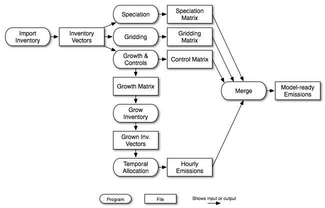
SMOKE is designed to take advantage of these facts by formulating emissions modeling in terms of sparse matrix operations, which can be performed by optimized sparse matrix libraries. Specifically, the inventory emissions are arranged as a vector of emissions sorted in a particular order, with associated vectors that include characteristics about the sources such as the state/county and SCCs. SMOKE then creates matrices that apply the control, gridding, and speciation factors to the vector of emissions. In many cases, these matrices are independent from one another, and can therefore be generated in parallel and applied to the inventory in a final “merge” step, which combines the inventory emissions vector (now an hourly inventory file) with the control, speciation, and gridding matrices to create model-ready emissions. Figure 2.4, “Parallel approach to emissions processing” shows how the matrix approach allows for a more parallel approach to emissions processing, in which fewer steps depend on other needed steps.

Note that in Figure 2.4, “Parallel approach to emissions processing”, temporal allocation outputs hourly emissions instead of a temporal matrix. This is because of some peculiarities with temporal modeling for point sources, which can use hourly emissions as input data. To be able to overwrite the inventory emissions with these hourly emissions, the temporal allocation step must output the emissions data. The matrix approach is used internally in the temporal allocation step.

The growth and controls steps shown in Figure 2.4, “Parallel approach to emissions processing” are optional. If the inventory is not grown to a future or past year, then the temporal allocation step uses the original inventory vectors to calculate the hourly emissions.

Several benefits can be realized from this more parallel approach. For example, given a single emissions inventory, temporal modeling is performed only once per inventory and episode (though in practice, this step is often performed once per episode day). Also, gridding matrices typically need only be calculated once per inventory and model grid definition, without having to reprocess other steps. As shown in Figure 2.5, “Processing steps for running an additional grid in SMOKE”, SMOKE usually needs to rerun only the gridding and merge steps to process a different grid for the same inventory. The merge step in the figure will read the previously created results from the temporal allocation, chemical speciation, and control processing steps.

In addition, speciation matrices need only be calculated once per inventory and chemical mechanism. Similar to the gridding example, Figure 2.6, “Processing steps for running an additional chemical mechanism in SMOKE” shows the SMOKE steps that generally need to be rerun for running an additional chemical mechanism.

A final example of how this approach is beneficial is processing with a control strategy. Because of SMOKE’s parallel processing, changing a control strategy requires only the control and merge steps to be processed again (Figure 2.7, “Processing steps for running a control scenario in SMOKE”). In serial processing, on the other hand, the growth and controls step occurs as the second processing step, which requires that all downstream steps be redone. In Figure 2.7, “Processing steps for running a control scenario in SMOKE”, the speciation, temporal allocation, and gridding steps have already been run, and can be fed to the merge step without being altered or regenerated.

Although SMOKE processing generally follows the structure shown in Figure 2.4, “Parallel approach to emissions processing”, there are some exceptions. In the list below, we summarize these exceptions and provide references to the sections of this chapter where these exceptions are explained and shown through diagrams. These exceptions are also described in more detail in Section 2.8.2, “Area-source processing”, Section 2.8.3, “Biogenic-source processing”, Section 2.8.4, “Mobile-source processing”, and Section 2.8.5, “Point-source processing”.