MOVES is the U.S. Environmental Protection Agency's (EPA)
Motor Vehicle Emission Simulator (OTAQ, 2009, also available at http://www.epa.gov/otaq/models/moves/index.htm
and). The purpose of MOVES is to provide an accurate estimate of emissions from
mobile sources under a wide range of user-defined conditions. It helps the user
answer "what if" questions, such as "How would particulate
matter emissions decrease in my state on a typical weekday if truck travel were
reduced during rush hour?", or "How does the total hydrocarbon
emission rate change if my fleet switches to gasoline from diesel fuel?"
In the modeling process, the user specifies vehicle types,
time periods, geographical areas, pollutants, vehicle operating
characteristics, and road types to be modeled. The model then performs a series
of calculations, which have been carefully developed to accurately reflect
vehicle operating processes (such as cold start or extended idle) and provide
estimates of bulk emissions or emission rates. Specifying the characteristics
of the particular scenario to be modeled is done by creating a Run
Specification, or runspec (discussed further in Section 3).
The outputs from MOVES are emissions estimates or emissions
factors. These can be used as inputs to larger emissions modeling systems that
model many different types of emissions (e.g., stationary point sources, area
sources and biogenic sources) and provide results that are used in performing
air quality modeling. An example of such systems is the Sparse Matrix Operator
Kernel Emissions (SMOKE) model, which is widely used in both the public and
private sectors (IE, 2009a). Detailed information about SMOKE is available at http://www.smoke-model.org.
In December 2009, a new version of MOVES was released: the
Motor Vehicle Emission Simulator 2010
model (MOVES2010). An important feature of MOVES2010 is that it allows users to
choose between (1) the “Inventory” calculation type, which provides emission
rates in terms of total quantity of emissions for a given time period; and (2) the
“Emission Rate” calculation type, which gives emission rates in terms of grams/mile
or grams/vehicle/hour. For large-scale emissions modeling such as that needed
for regional- and national-scale air quality modeling projects, it is desirable
to use the Emission Rate calculation type, which populates emission rate lookup
tables that can then be applied to many times and places, thus reducing the
total number of MOVES runs required.
Under Work Assignment (WA) 3-03 of EPA contract EP-D-07-102
to the University of North Carolina at Chapel Hill (UNC), EPA’s Office of
Transportation and Air Quality (OTAQ) has tasked UNC and ENVIRON with
developing tools to facilitate the process of using MOVES to create emissions
estimates appropriate for air quality modeling.
The successful use
of the MOVES Emission Rate calculation type requires careful planning and a
clear understanding of emission rates calculation in MOVES. To reduce the time
and effort required of the user for this process, and to help the user obtain
more accurate modeling results, UNC and ENVIRON created a new tool called the SMOKE-MOVES
integration tool (Figure 1). This tool consists of a set of scripts that
automate the proper use of the Emission Rate calculations for the purpose of
estimating mobile-source emissions for air quality (AQ) modeling. The
SMOKE-MOVES tool provides three major functions:
1.
Meteorological data preprocessor:
·
The
meteorological data preprocessor program (Met4moves) prepares spatially and
temporally averaged temperatures and relative humidity data to set up the
meteorological input conditions for MOVES and SMOKE using the Meteorology-Chemistry
Interface Processor (MCIP) output files.
2. MOVES
model processing:
·
The
MOVES driver script creates data importer files and the MOVES input file
(runspec), which specifies the
characteristics of the particular scenario to be modeled.
·
The MOVES
postprocessing script formats the MOVES emission rate lookup tables for
SMOKE.
3. SMOKE
model processing:
·
The SMOKE postprocessing program (Movesmrg)
estimates emissions from on-road mobile sources based on MOVES-based emission rate
lookup tables and meteorology data from Met4moves.
·
Creates hourly gridded speciated air quality
model-ready input files.
·
Produces various types of reports for users.
This user’s guide
describes the major functions of the SMOKE-MOVES integration tool.
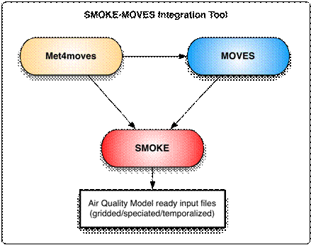
Figure 1. Flow diagram of
overall SMOKE-MOVES integration tool.
Before we provide more information about the tool, this
section discusses some key concepts and terminology that will help users in understanding
this document.
Reference county – The approach for
running MOVES for SMOKE relies on the concept of reference counties. These are
counties that are used during the
creation and use of emission rates to represent a set of similar counties
(i.e., inventory counties) called a county
group. The purpose of the reference county is to reduce the computational
burden of running MOVES on every county in your modeling domain. By using a
reference county, the user generates key emission rates for the single county
in MOVES and then utilizes these factors to estimate emissions for all counties
in the county group through SMOKE. The reference county is modeled at a range
of speeds and temperatures to produce emission rate lookup tables (grams/mile
or grams/vehicle/hour, depending on mobile emission process). The variables
that are assumed to be constant across the county group members (and the
reference county) are fuel parameters, fleet age distribution and
inspection/maintenance (I/M) programs. The variables that can vary within the
county group are vehicle miles traveled (VMT), source type vehicle population,
roadway speed, and grid cell temperatures. Determining the reference counties
and their respective county groups is a key aspect of utilizing the SMOKE-MOVES
tool. It is ideal for the user to create each county group based on the
similarity between the county characteristics (e.g., urban and rural) and the
meteorological conditions (e.g., temperature and relative humidity). The user
should avoid grouping counties that have significantly different meteorological
conditions.
Fuel month – The concept of a fuel month is used to indicate when a
particular set of fuel properties should be used in a MOVES simulation. Similar
to the reference county, the fuel month reduces the computational time of MOVES
by using a single month to represent a set of months. To determine the fuel
month and which months it corresponds to, the user should review the
State-provided fuel supply data in the MOVES database for each reference
county. If the fuel supply data change throughout the year, then group the
months by fuel parameters. For example, if the grams/mile exhaust emission
rates in January are identical to February’s rates for a given reference
county, then use a single fuel month to represent January and February. In
other words, only one of the months needs to be modeled through MOVES.
When the MOVES model runs as a part of the SMOKE-MOVES tool,
it runs for all emissions processes (or modes), including on-road and
off-network emissions processes, for the selected pollutants. Off-network
emission processes (e.g., parked engine-off, engine starts, and idling, and
fuel vapor venting) in MOVES are hour-dependent due to vehicle activity
assumptions built into the MOVES model; the emission rate depends on both hour
of the day and temperature. On-roadway emission processes (e.g., running
exhaust, crankcase running exhaust, brake wear, tire wear, and on-road
evaporative), on the other hand, do not depend on hour. In MOVES, these
emission processes are categorized into three major groups:
- rate-per-distance (RPD) – The emission rate of vehicles on-network (i.e., driving) from MOVES.
The rate is expressed in grams/mile traveled.
- rate-per-vehicle (RPV) – The
emission rate of vehicles off-network (e.g., idling, starts, refueling,
parked) from MOVES. The rate is given in grams/vehicle/hour.
- rate-per-profile (RPP) – The
emission rate of vehicles off-network—specifically, the evaporation from
parked vehicles (vapor-venting emissions) from MOVES. The rate is
expressed in grams/vehicle/hour.
This SMOKE-MOVES integration tool user’s
guide assumes that readers have some experiences using both the MOVES model and
the SMOKE model; this type of knowledge is necessary for effective use of the
SMOKE-MOVES tool. For detailed information about these models, please check
their user’s guides (OTAQ, 2009; IE, 2009a).
Met4moves is a meteorological preprocessor that prepares
temperature and relative humidity (RH) data for use by both MOVES and SMOKE
(see Figure 2). Met4moves produces specific meteorological metrics for the
reference county(s) for MOVES and additional meteorological metrics for all
inventory counties in the county group for SMOKE. The meteorological metrics
are specific to the emissions processes (RPD, RPV, or RPP); this is discussed
in more detail below.
The inputs for Met4moves include the reference county
cross-reference file (MCXREF), the reference county fuel month cross-reference
file (MFMREF) for mapping reference counties to fuels and months, spatial
surrogates used to identify grid cells per county (SRGLIST), a list of counties
(COSTCY), the grid description (GRIDDESC), and gridded hourly temperatures
output from MCIP (ORD, 2009). More information about the inputs for Met4moves
is available in Section 2.3.1.
The outputs are (1) a file for MOVES that contains the
temperatures and RH for each reference county, and (2) a file for SMOKE that
contains the temperatures and RH for each inventory county in the county
group(s), supplementing the gridded hourly temperatures from MCIP. More
specifically:
·
For MOVES, Met4moves creates datasets that
provide all minimum/maximum (min/max) temperature combinations for a reference
county, reflecting all min/max combinations for all inventory counties in that
county group. The associated RH values are also included in these datasets. In
addition, the datasets include the 24-hour diurnal profiles needed for the RPP emission
process, and contain user-specified temperature increments for use by MOVES.
This is discussed in more detail at Section 2.3.3.1.
·
For SMOKE, Met4moves creates datasets that
contain the min/max temperatures, and averaged RH associated for each inventory
county. More detailed information is available in Section 2.3.3.2.
The key difference between the datasets provided to MOVES
and those provided to SMOKE is that the former includes only the reference
counties, while the latter includes all of the inventory counties.
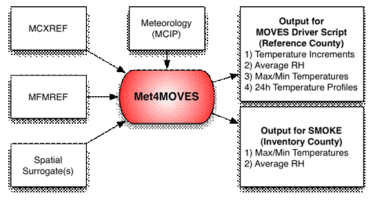
Figure 2. Flow diagram of
Met4moves
As described in Section 1.1.1, the SMOKE-MOVES approach is based on reference counties, each one
representing a county group that shares the same fuel parameters, fleet age
distribution, I/M programs, and meteorological conditions. The use of reference
counties allows reductions in the MOVES processing time and in the sizes
of the emission rate lookup tables.
The reference county cross-reference
file (MCXREF) defines the reference
counties, and the county group that maps to each reference county. Table 1
provides the format for this input file, while Table 2 gives an example of
reference county cross-reference file entries (both of these tables are shown
later in Section 2.3.1.4).
2.1.3
Spatial Averaging Method for Temperature and
RH Data
In order to combine gridded meteorology data with
county-based mobile emissions data, a technique has been developed for
calculating spatially averaged meteorology for each reference county. Because
not all of the grid cells in a county contain on-road mobile emissions, this
technique provides a way to select which cells should be used in determining
the min/max temperatures and 24-hour temperature profiles. Spatial surrogates
(see IE, 2009b) are used to select grid cells in each county group where the
mobile emissions are located. Based on the definitions of reference counties
and county groups, and the specific spatial surrogates, Met4moves selects the
appropriate meteorology grid cells across the county groups. It uses the
temperatures in the selected grid cells to create the temperature input files
for both the MOVES model (using a process described in Section 3) and the SMOKE
model (using a process described in Section 4). Details of defining a subset of
county grid cells for MOVES modeling include the following:
·
The user must specify at least one spatial
surrogate for Met4moves processing.
·
Using more than one surrogate could provide a
proxy for grid cells with higher mobile emission activities.
·
To select all grid cells within the county, the
user could select a total land area surrogate.
·
The grid cells selected will likely vary
depending on the choice of spatial surrogate(s).
·
Only the selected grid cells are used to
estimate the min/max temperatures and 24-hour temperature profiles.
·
When selecting the absolute min/max temperatures
in any hour that are needed for the reference county, Met4moves considers all
the selected grid cells in the reference county and all the selected grid cells
from inventory counties in the county group. This approach is needed because
the reference county could have a smaller temperature range than one of the
counties that is mapped to it. The absolute min/max temperatures are used for
computing RPD and RPV emissions processes.
·
When calculating the diurnal temperature 24-hour
profiles for the reference county, Met4moves considers all the selected grid
cells in the reference county and all the selected grid cells from inventory
counties in the county group. This approach is needed because the reference
county could have a smaller temperature range than one of the counties that is
mapped to it. The 24-hour diurnal shape profiles are used for computing various
24-hour diurnal profiles based on min/max temperature combinations for the RPP
emissions process.
Met4moves uses hourly min/max temperatures and averaged RH
over the spatial region that includes all of the inventory counties in a county
group over the user-defined modeling period. The current version of Met4moves
supports only the monthly averaging method (versus daily or episodic) to create
min/max temperatures and averaged RH for all inventory counties in the county
group(s). This means, for example,
that if you process an entire year using the monthly averaging method, then
Met4moves will produce 12 calendar months of min/max temperatures and averaged
RH for all of the inventory counties in the county group for SMOKE.
When computing RH, Met4moves defaults to using only the
hours from 6 AM through 6 PM, in order to exclude hours with little traffic
that would artificially skew the values. Users can override the default and
change the hours of the day to use for this calculation, if desired. Detailed
information for this setting is available in Section 2.3.2.
As described in Section 1.1.1, the concept of a fuel month
is used to indicate when a particular set of fuel properties should be used in
a MOVES simulation. To group months by fuel properties, the user must create and input a fuel month file
(MFMREF) to Met4moves. The fuel month file is a text file that contains
reference county FIPS codes, monthly fuel type identification (ID) codes, and
the months that use each fuel type (Tables 3 and 4, shown later in Section
2.3.1.5). If a fuel month file
containing more than one fuel month entry is provided to Met4moves, fuel-month-specific
temperature outputs will be created for the MOVES model. For example, if a
reference county has four fuel months representing the entire year with the
monthly averaging method, then Met4moves will produce four sets of temperatures
and averaged RH outputs for the reference county, as opposed to 12 calendar
months of outputs for the county group. The outputs for the reference county
are used as input to the MOVES driver script (Section 3), while the outputs for
the county group are used as input for SMOKE processing (Section 4).
Temperature increments are used by MOVES to determine the
number of emission rates needed in the various lookup tables. The user can
define three different temperature increments, which control the RPD, RPV, and
RPP emissions processes, respectively. MOVES will calculate emission rates at
the various temperatures (determined by the temperature increment) and bounded
by the range of absolute min/max temperatures. This provides some control over
the number of MOVES runs. Note that all temperatures produced by Met4moves are
in ºF.
Examples: If the
absolute min/max for an averaging period and reference county is 68/94 ºF,
the temperatures associated with the RPD, RPV, and RPP calculations are as
follows:
a. For
RPD, a temperature increment of 5 ºF would require emission rates at all
temperature from 65 ºF to 95 ºF in 5º increments.
b. For
RPV, a temperature increment of 10 ºF would require emission rates for each
hour at 60, 70, 80, 90, and 100 ºF. (Note that these are needed for each hour
because RPV depends on hour of day as well as temperature.)
c. For
RPP, with a temperature increment of 10 ºF, Met4moves will create a set of
24-hour temperature profiles based on the normalized 24-hour shape profile.
This set of profiles will cover all combinations of min/max values within the
absolute min/max range. In this example, the set of profiles (min, max) are:
(60, 100), (70, 100), (80, 100), (90, 100), (100,100), (60, 90), (70, 90), (80,
90), (90,90), (60, 80), (70, 80), (80,80), (60, 70), (70,70), and (60, 60) ºF.
2.2 Met4moves
Processing
Using the specified county groups and temporal averaging
approach for temperature and RH data (Section 2.1.4), Met4moves determines the
min/max grid cell temperatures and associated RH for both SMOKE and MOVES, and
computes average 24-hour temperature profiles for use in MOVES.
The 24-hour temperature profiles are averaged over a
user-specified time period and grid cells for the reference county. Each
profile is assigned to a profile ID code that identifies the combination of
minimum and maximum temperatures. Note that there could be several temperature
profile IDs used by the MOVES driver scripts (discussed in Section 3) for a
single iteration of MOVES.
2.2.2
Met4moves Processing Sequence
Met4moves must be run on a Linux / Unix computer after
running MCIP and before running MOVES and SMOKE.
The following are the major processing steps that Met4moves
performs:
1. Read
the reference county cross-reference file (MCXREF) that contains a list of
reference counties and the county groups that map to those reference counties.
2. Read
the surrogate description file (SRGDESC) and a list of associated spatial
surrogate(s) chosen for use in selecting grid cells.
3. Determine
a list of grid cells for each county. Only the selected grid cells are used to
estimate the min/max temperatures, 24-hour temperature profiles, and RH over
the user-specified modeling period.
4. Set the dates of the modeling episode in local time using
the flags STDATE and ENDATE.
5. Determine
the averaging method (AVERAGING_METHOD)
chosen by the user to create 24-hour temperature profiles (i.e., MONTHLY).
6. Determine the fuel month for the reference
county using the MFMREF input file.
7. Read
the country/state/county (COSTCY) file to define the time zones for county
groups.
8. Read
the meteorology data that have been processed by MCIP.
9. Calculate
the min/max temperatures hourly and over the modeling period.
10. Calculate
average RH for the specified hour range over the modeling period. The default
hour range is from 6 AM to 6 PM local time).
11. Once
min/max temperatures and averaged RH are estimated for all reference counties
and all inventory counties in the county groups, estimate diurnal 24-hour
temperature profiles for use by the MOVES driver script (Section 3). The result
is a normalized 24-hour shape profile over the user-specified period or fuel
month.
2.3 Files
and Environment Variables for Met4moves
Met4moves requires several input files (Figure 3). This
includes the reference county cross-reference file (MCXREF), the reference
county fuel month cross-reference file (MFMREF) for mapping reference counties
to fuels and months, spatial surrogates used to identify grid cells per county
(SRGLIST), a list of counties (COSTCY), the grid description (GRIDDESC), and
gridded hourly temperatures MCIP output.
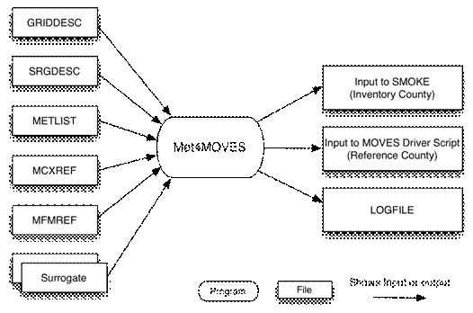
Figure 3. A flow diagram of
Met4moves input and output files.
2.3.1.1 GRIDDESC: Grid Description File
The GRIDDESC input file describes the modeling grid. See
the SMOKE user’s manual (http://www.smoke-model.org)
for details.
2.3.1.2 SRGDESC: Surrogate Description File
The SRGDESC input file includes a surrogate list,
description, and surrogate file name used in the modeling grid. Note: The user
must set SRGPRO_PATH to define the location of the spatial surrogate
coefficient file(s). See the SMOKE user’s manual for details.
2.3.1.3 METLIST:
Spatial Surrogate File
The METLIST input file contains a list of MCIP meteorology
files, including their full paths.
2.3.1.4 MCXREF: Reference county cross-reference File
The MCXREF input
file defines the reference counties, and the county group that maps to
each reference county. In defining the reference counties and county groups,
the following guiding principles should be taken into account:
·
The members of the county group should have the
same fuel characteristics, the same distribution of fuels over the year, the
same I/M programs, and the same fleet age distribution.
·
Since RH is averaged over a county group,
grouping counties with reasonably similar daytime RH is advisable.
·
Since min/max temperature and diurnal
temperature profiles are calculated over a county group, grouping counties with
reasonably similar temperature ranges is advisable. Optionally, the shape of
the diurnal temperature distribution can be considered for defining county
groups. The shape of the diurnal temperature profile is created based on
intersections with all inventory counties in the county group.
·
Optionally, the ratio of VMT to vehicle
population can be considered in the definition of county groups, since the
ratio affects the off-network emissions factors. This could be a minor factor
in the county grouping, but it would be incomplete not to mention it.
The MCXREF
file is a comma-separated-values (CSV) file. Table 1 provides the file format,
and Table 2 gives an example set of entries for this file. The user can either
include or exclude leading zeroes. For example, California could be represented
by ‘06’ or ‘6’.
Table 1. Format of reference county cross-reference
file (MCXREF)
|
Line
|
Col
|
Description
|
|
1+
|
A
|
One-digit country FIPS code for inventory county (Integer)
|
|
|
B
|
Two-digit state FIPS code for inventory county (Integer)
|
|
|
C
|
Three-digit
county FIPS code for inventory county (Integer)
|
|
|
D
|
One-digit country FIPS code for reference county (Integer)
|
|
|
E
|
Two-digit state FIPS code for reference county (Integer)
|
|
|
F
|
Three-digit
county FIPS code for reference county (Integer)
|
Table 2. Example of
reference county cross-reference file entries
|
County Groups
|
Reference Counties
|
|
Country
|
State
|
County
|
Country
|
State
|
County
|
|
0
|
13
|
101
|
0
|
|
121
|
|
0
|
13
|
102
|
0
|
13
|
121
|
|
0
|
13
|
103
|
0
|
13
|
121
|
|
…
|
…
|
…
|
…
|
…
|
…
|
|
0
|
13
|
121
|
0
|
13
|
121
|
|
0
|
13
|
123
|
0
|
13
|
217
|
|
0
|
13
|
125
|
0
|
13
|
217
|
|
0
|
13
|
127
|
0
|
13
|
217
|
|
…
|
…
|
…
|
…
|
…
|
…
|
2.3.1.5 MFMREF:
Reference County Fuel Month File
The MFMREF input
file serves the purpose of grouping months of the year by fuel
parameters. The file specifies representative fuel months (the fuelMonth field in
the MOVES database) to assign to the calendar months being simulated (the Month
field) for each reference county.
As with MCXREF,
MFMREF is a CSV file. Table 3 provides the file format. Table 4 is an example
that illustrates a situation in which there are three fuel formulations in a
given calendar year to be modeled in SMOKE-MOVES. In this example, reference
county 13121 uses the fuel formulation mix in January (1) for modeling months November
(11), December (12), January (1) and February (2). The April (4) fuel
formulation mix is used for March (3), April (4), and May (5). The June (6)
fuel formulation mix is used for simulating June (6), July (7), August (8),
September (9), and October (10). The user can either include or exclude leading
zeros for the country codes; for example, USA country code ‘0’ could be
excluded.
Table 3. Format of reference county fuel month file
(MFMREF)
|
Line
|
Position
|
Description
|
|
1+
|
A
|
Six-digit county-specific code for reference county
(Integer)
|
|
|
fuelMonth
|
Reference county fuel month (Integer)
|
|
|
Month
|
Month
(Integer)
|
Table 4. Example of reference county fuel month
file entries
|
RefCounty
|
fuelMonth
|
Month
|
|
013121
|
1
|
1
|
|
013121
|
1
|
2
|
|
13121
|
4
|
3
|
|
13121
|
4
|
4
|
|
13121
|
4
|
5
|
|
13121
|
6
|
6
|
|
13121
|
6
|
7
|
|
13121
|
6
|
8
|
|
13121
|
6
|
9
|
|
13121
|
6
|
10
|
|
13121
|
1
|
11
|
|
13121
|
1
|
12
|
Environment variables are used to provide settings to
Met4moves that control the functioning of the program. These settings are
below.
·
STDATE: [default: 0]
Sets the
overall episode start date; Julian format (YYYYDDD).
·
ENDATE: [default: 0]
Sets the
overall episode end date; Julian format (YYYYDDD).
·
AVERAGING_METHOD:
[default: MONTHLY]
Sets
averaging method to create 24-hour temperature profiles based on STDATE and ENDATE
o
MONTHLY: Average
data and profiles for each month within the user-specified modeling episode.
MONTHLY is the only allowable method at this time.
·
MOVES_OUTFILE:
[default: none]
Defines the output filename for MOVES.
·
SMOKE_OUTFILE:
[default: none]
Defines the output filename for SMOKE.
·
PD_TEMP_INCREMENT:
[default: 5]
Defines the temperature increment (in
ºF) for RPD lookup table (described in Section 3.1.1.2) to create combinations
of min/max temperature bins.
·
PV_TEMP_INCREMENT:
[default: 5]
Defines the temperature increment (in
ºF) for RPV lookup table (described in Section 3.1.1.2) to create combinations
of min/max temperature bins.
·
PP_TEMP_INCREMENT:
[default: 10]
Defines the temperature increment (in
ºF) for RPP lookup table (described in Section 3.1.1.2) to create combinations
of min/max temperature bins for normalized 24-hour diurnal temperature profile.
·
RH_STR_HOUR:
[default: 60000]
Defines the start hour in local time for
average RH over the user-specified modeling episode.
·
RH_END_HOUR:
[default: 180000]
Defines the end hour in local time for
average RH over the user-specified modeling episode.
·
SRG_LIST:
[default: none]
Specifies the name(s) of the spatial
surrogate(s) to be used in selecting the grid cells for the county (example:
setenv SRG_LIST ‘100, 230’).
·
SRGPRO_PATH:
[default: none]
Defines the location of spatial
surrogate coefficient files.
·
TMPVNAME:
[default: TEMP2]
Specifies the variable name for the
temperature to extract from MCIP files.
Met4moves produces two output files (Figure 3). The main
difference between the output files is that the output file created for input
to the MOVES driver script (Section 3) includes data for the reference counties
only, while the output file created for input to SMOKE includes data for all of
the counties within the modeling domain.
2.3.3.1
MOVES_OUTFILE: Output File for MOVES Driver
Script
The
output file created for use by the MOVES driver script contains the absolute
minimum and maximum temperatures and average RH values associated with each
reference county. The scope of these min/max temperatures extends across the
selected grid cells in the county group associated with that reference county.
The min/max temperatures determine the MOVES runs that are needed for
generating the RPD and RPV emission rates. The temperature increments listed in
the header are used to define the temperature bins used to optimize the MOVES
runs (Table 5). In addition, the output file prepared for the MOVES driver
script contains sets of diurnal temperature profiles based on combinations of
min/max temperature bins for each reference county; these are necessary for the
MOVES vapor-venting emissions calculation that is performed for the RPP
emissions process.
This output
file contains all of the temperature and RH values for all reference counties.
If, for example, the duration of the episode is annual, there are four fuel
months, and the averaging method is monthly, Met4moves outputs four sets of
monthly average RH, min/max temperatures, and 24-hour temperature profiles in
local time for all reference counties into one output file. An example of this
file is provided in Table 5. When each set of fuel month min/max temperatures
begins with the record “min_max” in the temperatureProfileID column, the “Temp1”
and “Temp2” fields can be referred to as minimum and maximum temperatures,
respectively. The remaining records for the specific reference county and fuel
month (the records between this “min_max” and the next “min_max”) are the
24-hour temperature profiles. The profile names, temperatureProfileID, are a
combination of the averaging type (M is for monthly), the last Julian date of
the averaging period, and an index of the profiles (e.g., M2009180003 is the
third monthly profile for the 2009180 averaging period). For a specific
reference county and fuel month, the monthly average RH value is identical for
all the records.
Table 5. Format of reference
county minimum/maximum temperatures, relative humidity, temperature increments,
and temperature profiles used as input to MOVES driver script
|
#
DESC Sample Met input file for MOVES Driver script
PD_TEMP_INCREMENT
5
PV_TEMP_INCREMENT
5
PP_TEMP_INCREMENT
10
|
|
Ref.
County
|
fuelMonth
|
temperatureProfileID
|
RH
|
Temp1
(Min)
|
Temp2
(Max)
|
Temp3
|
…
|
Temp24
|
|
13121
|
1
|
min_max
|
66.82
|
31.21
|
89.98
|
|
|
|
|
13121
|
1
|
M2009120001
|
66.82
|
37.80
|
35.69
|
34.50
|
…
|
41.07
|
|
13121
|
1
|
M2009120002
|
66.82
|
46.50
|
44.75
|
43.75
|
…
|
49.23
|
|
13121
|
1
|
M2009120003
|
66.82
|
55.20
|
53.80
|
53.00
|
…
|
57.38
|
|
…
|
…
|
…
|
…
|
…
|
…
|
…
|
…
|
…
|
|
13121
|
4
|
min_max
|
66.21
|
45.21
|
90.2
|
|
|
|
|
13121
|
4
|
M2009180001
|
66.21
|
47.88
|
45.12
|
44.52
|
…
|
51.06
|
|
13121
|
4
|
M2009180002
|
66.21
|
56.51
|
54.45
|
53.35
|
…
|
59.24
|
|
13121
|
4
|
M2009180003
|
66.21
|
65.94
|
63.55
|
63.15
|
…
|
67.65
|
|
…
|
…
|
…
|
…
|
…
|
…
|
…
|
…
|
…
|
2.3.3.2
SMOKE_OUTFILE: Output File for the SMOKE Model
The
output file created for use by the SMOKE model contains county-specific min/max
temperatures and averaged RH values in local time for every inventory county
and averaging period in the modeling inventory. Table 6 gives an example of
this file. SMOKE adjusts the native MCIP time zone (GMT) to local time in order
to properly use the Met4moves lookup tables, which are given in local time.
This output contains the actual month (Month), the fuel month (fuelMonth) and
the Julian date (julianDate) used by MOVES to generate the emission rate lookup
tables. If the averaging method is set to monthly, julianDate will contain the
last Julian date of the averaging month. There are no 24-hour profiles, since
SMOKE does not need them.
Table 6. Format of inventory
county-specific minimum/maximum temperatures
and temperature profiles used as input to SMOKE.
|
Inventory
County
|
fuelMonth
|
Month
|
julianDate
|
RH
|
Temp
(Minimum)
|
Temp
(Maximum)
|
|
13001
|
1
|
3
|
2009060
|
51.1
|
25.2
|
65.1
|
|
13002
|
1
|
3
|
2009060
|
55.2
|
29.1
|
58.9
|
|
13003
|
1
|
3
|
2009060
|
52.6
|
21.4
|
59.3
|
|
13005
|
1
|
3
|
2009060
|
51.7
|
25.8
|
62.1
|
|
…
|
…
|
…
|
…
|
…
|
…
|
…
|
|
13001
|
4
|
4
|
2009090
|
61.1
|
44.2
|
75.1
|
|
13002
|
4
|
4
|
2009090
|
66.6
|
39.9
|
63.7
|
|
13003
|
4
|
4
|
2009090
|
61.1
|
45.1
|
80.5
|
|
13005
|
4
|
4
|
2009090
|
56.2
|
46.2
|
79.5
|
|
…
|
…
|
…
|
…
|
…
|
…
|
…
|
3 MOVES Model Processing
The second major component of the SMOKE-MOVES tool is MOVES model processing. This involves
two scripts: The MOVES driver script (Section
3.1) creates data importer files and the MOVES input file (runspec),
which specifies the characteristics of
the particular scenario to be modeled. The MOVES postprocessing script (Section
3.2) formats the MOVES emission rate lookup tables for SMOKE.
Unlike the Met4moves meteorology preprocessor and the SMOKE
modeling system, the MOVES driver script is typically run on Windows XP/Vista/7.
However, a version that can run on Linux may become available later in 2010
After you finish running Met4moves (Section 2) on Linux, you must copy the
Met4moves output file to system on which you are running MOVES (typically a
Windows computer). Next, run the MOVES driver script to perform the MOVES runs
and the postprocessing script to process the data output from MOVES on that
system to create the MOVES-based lookup tables.
These tables will be used as inputs to SMOKE that runs on Linux.
When you run the MOVES driver script, it generates the MOVES
driver files (both run specifications and data importers) based on the Met4moves
output temperature list by reference county, as follows:
- Reads the output file
from Met4moves and two other user input files.
- Assembles instructions
for MOVES to create MySQL input databases from XML files (data importer).
- Assembles run
specification (runspec) XML files to run MOVES for a wide range of
conditions.
- Generates the
run-specific temperature and humidity CSV file.
- Assembles a batch list
of data importer files, runspec files, and also a list of the MySQL.
output database names to be postprocessed.
Once the MOVES driver script has completed, the postprocessor script extracts the emissions
factor tables from the MOVES databases; maps MOVES source, fuel, and road types
to Source Classification Codes (SCCs); and formats the emissions factor tables
for use as SMOKE inputs, as follows:
- Reads the list of
databases created by the MOVES driver script.
- Maps from the MOVES
source types, fuel types, and road types to SCC, and aggregates SCC
emissions factors over model years.
- Performs operations to
drop and add fields and reduce the database size by performing a cross-tab
query that places all pollutants on a single row.
- Writes final processed
lookup tables to CSV files that are formatted for SMOKE.
3.1 MOVES Driver Script
The MOVES driver script, which is written in Perl, generates
outputs for each reference county. The goals of the driver script are (1) to
create the MOVES input files called “runspecs”; (2) to create all required
MOVES data importer files, which are the instructions to MOVES on how to build
county-level MySQL input databases; and (3) to create batch files of MOVES
commands that run MOVES from the Windows command prompt. When the user launches
the importer batch file though the Windows command prompt, the MOVES model
imports data files into MySQL tables, after which the user needs to launch the
runspec batch file so that MOVES calculates emission rates for all the conditions
specified in the runspecs.
This section of the user’s guide describes how to coordinate
the use of input data from Met4moves and raw MOVES inputs (e.g., prepared by
States or EPA) to create and organize the runspec files, and how to choose some
user selections (e.g., calendar year, pollutants of interest) and modify hard-coded
features (e.g., inclusion of all required emission processes for a given
pollutant).
The MOVES model can be run at any of the three
domains/scales: national, county, or project. Refer to the MOVES2010 user’s
guide for detailed descriptions of the different scales. The SMOKE-MOVES tool always
uses the county domain/scale because this level of model detail is required by
EPA for SIP and conformity analyses. For this scale, MOVES requires a MySQL
input database containing local data for a single county. Every runspec file
contains the name of a MySQL input database.
The MOVES driver script requires the following four types of
inputs:
1. A
run control file containing basic user selections for MOVES (example format in
Appendix A)
2. Meteorological
outputs from the Met4moves preprocessor for each reference county and fuel
month:
a.
Minimum and maximum temperatures
b.
Average daytime relative humidity
c.
Multiple sets of 24-hour temperature profiles
d.
Temperature increments
3. Reference
county file indicating the filenames by file type keyword for each of the files
specified in item 4 (see example format in Appendix A).
4. Reference
county inputs in CSV files formatted for the County Data Manager in MOVES that
specify:
a.
Vehicle age distribution
b.
Fuels (parameters and market shares, by month)
c.
I/M programs
d.
VMT
e.
Vehicle population
Using the MOVES driver script involves two major processing
steps: creation of the runspec files (Section 3.1.1), and user preparation of
the data inputs needed for using the driver script to assemble the MySQL input
data tables (Section 3.1.2). After the driver script approach is explained,
Section 3.2 describes the MOVES postprocessing script that is used with output
from a MOVES batch file run to generate the SMOKE-ready lookup table input
files.
The first action of the driver script is to create runspec
files for MOVES that contain all of the selections required to execute a run. The
MOVES driver script requires as input two files: a run control file in which
the user specifies calendar year, pollutants, and day type (weekday or
weekend); and the Met4moves output temperature file for the batch run of MOVES.
The user selections in the run control file determine the information printed
by the driver script in runspec files for MOVES.
3.1.1.1 Specifying
Pollutants
The user must specify in the run control file one or more
groups of pollutants to model. There are four groups available: ozone
precursors, toxics, PM, and greenhouse gases (GHG). The MOVES pollutants and
pollutant groups for the four types of modeling are provided below in Table 7.
The choice of pollutant group(s) determines what pollutants are included in the
three emission rate lookup tables output by MOVES (RPD, RPV, and RPP),
which are described in Section 3.3. The letter ‘X’ marks the key pollutants for
inclusion, and a ‘d’ signifies that the pollutant is included in the MOVES run
because a key pollutant depends on it.
Table 7. MOVES Pollutants Available for Inclusion
in the Lookup Tables Output by MOVES
|
pollutantID
|
pollutantName
|
Pollutant
group
|
|
Ozone
|
Toxics
|
PM
|
GHG
|
|
1
|
Total Gaseous Hydrocarbons
|
d
|
d
|
d
|
|
|
79
|
Non-Methane Hydrocarbons
|
d
|
d
|
d
|
|
|
80
|
Non-Methane
Organic Gases
|
d
|
d
|
d
|
|
|
86
|
Total
Organic Gases
|
X
|
X
|
X
|
|
|
87
|
Volatile
Organic Compounds
|
X
|
X
|
X
|
|
|
2
|
Carbon
Monoxide (CO)
|
X
|
|
|
|
|
3
|
Oxides
of Nitrogen
|
X
|
|
X
|
|
|
30
|
Ammonia
(NH3)
|
|
|
X
|
|
|
32
|
Nitrogen
Oxide
|
X
|
|
X
|
|
|
33
|
Nitrogen
Dioxide
|
X
|
|
X
|
|
|
31
|
Sulfur
Dioxide (SO2)
|
|
|
X
|
|
|
100
|
Primary
Exhaust PM10 – Total
|
|
d
|
X
|
|
|
101
|
Primary
PM10 - Organic Carbon
|
|
d
|
X
|
|
|
102
|
Primary
PM10 - Elemental Carbon
|
|
d
|
X
|
|
|
105
|
Primary
PM10 - Sulfate Particulate
|
|
d
|
X
|
|
|
106
|
Primary
PM10 - Brakewear Particulate
|
|
|
X
|
|
|
107
|
Primary
PM10 - Tirewear Particulate
|
|
|
X
|
|
|
110
|
Primary
Exhaust PM2.5 - Total
|
|
|
X
|
|
|
111
|
Primary
PM2.5 - Organic Carbon
|
|
|
X
|
|
|
112
|
Primary
PM2.5 - Elemental Carbon
|
|
|
X
|
|
|
115
|
Primary
PM2.5 - Sulfate Particulate
|
|
|
X
|
|
|
116
|
Primary
PM2.5 - Brakewear Particulate
|
|
|
X
|
|
|
117
|
Primary
PM2.5 - Tirewear Particulate
|
|
|
X
|
|
|
91
|
Total
Energy Consumption
|
|
d
|
d
|
X
|
|
92
|
Petroleum
Energy Consumption
|
|
|
|
X
|
|
93
|
Fossil
Fuel Energy Consumption
|
|
|
|
X
|
|
5
|
Methane
(CH4)
|
d
|
d
|
d
|
X
|
|
6
|
Nitrous
Oxide (N2O)
|
|
|
|
X
|
|
90
|
Atmospheric
CO2
|
|
|
|
X
|
|
98
|
CO2
Equivalent
|
|
|
|
X
|
|
20
|
Benzene
|
|
X
|
X
|
|
|
21
|
Ethanol
|
|
|
|
|
|
22
|
MTBE
|
|
X
|
|
|
|
23
|
Naphthalene
|
|
X
|
|
|
|
24
|
1,3-Butadiene
|
|
X
|
|
|
|
25
|
Formaldehyde
|
|
X
|
|
|
|
26
|
Acetaldehyde
|
|
X
|
|
|
|
27
|
Acrolein
|
|
X
|
|
|
3.1.1.2 Driver
Script Approach for Organizing Emission Processes
When the MOVES driver script creates the runspec files, it
includes all emissions processes (or modes) for the selected pollutants. To
optimally implement this design, different emission processes are selected in
separate runspecs but sent to the same output database of lookup tables. The
remainder of this subsection explains the grouping of emissions processes (RPD,
RPV, RPP).
For RPD lookup tables: Off-network emission
processes in MOVES are hour-dependent due to vehicle activity assumptions
built into the MOVES model; the emission rate depends on both hour of the day
and temperature. On-roadway emission processes, on the other hand, do not
depend on hour. Thus, the total MOVES run time can be reduced by implementing
the temperatures of interest in hour spots for the on-road running processes.
The MOVES driver script therefore groups together the on-roadway emission
processes that occur in a single runspec file. Processes that fall into this
category include the following:
Running
Exhaust
Crankcase
Running Exhaust
Tire
Wear
Brake
Wear
On-road
Evaporative Permeation (roadTypeID=2,3,4,5)
On-road
Evaporative Fuel Leaks (roadTypeID=2,3,4,5)
On-road
Evaporative Vapor Venting (roadTypeID=2,3,4,5)
These processes have in common that they have no dependence
on hour of the day and their emission rates are all written to the RPD lookup
table in grams/mile traveled. Due
to the lack of dependence on hour of the day, individual temperature bins in
the min/max temperature range can be placed in hours 1 through 24 sequentially.
For emission rate calculation, MOVES automatically generates the emission rates
for all 16 speed bins (see Table 9) at every temperature bin. The temperature
increment (#PR_TEMP_INCREMENT) used to divide temperature bins between the
minimum and maximum is provided through the header of the Met4moves temperature
preprocessor (Table 5). Potentially, there could be more than 24 temperature
bins, in which case a second runspec file for these processes would be created.
For RPV lookup tables: The second grouping of
emission processes occur from parked cars. These are run together in a MOVES
runspec file for the same reference county. The emission processes in this
grouping are listed below.
Start
Exhaust
Crankcase
Start Exhaust
Off-network Evaporative Permeation (roadTypeID=1)
Off-network Evaporative Fuel Leaks (roadTypeID=1)
Crankcase Extended Idle Exhaust
Extended Idle Exhaust
The MOVES emission rates for these processes are all written
to the RPV lookup table and have units of grams/vehicle/hour. The rates depend
on hour for various reasons. Start exhaust depends on engine soak time, which
varies by hour. Additionally, the lookup table hourly emission rates already
incorporate an assumption about the number of starts per vehicle by hour. Similarly,
for off-network evaporative emissions and extended idle exhaust, hourly
emission rates contain activity assumptions for parked time and idling time
activity. As such, this group of emission processes must be run at a single
temperature for each of the 24 hours of the day, and the entire range of
temperatures will be modeled by using a separate runspec file for each
temperature. The number of runspec files equals the number of temperature
increments (#PV_TEMP_INCREMENT) (Table 5). MOVES does not calculate these
processes at different speeds.
For RPP lookup tables: The third and final
group of emissions processes needing its own runspec file for the same reference
county includes just one process: off-network evaporative fuel vapor venting.
This emission rates for this process are written to the RPP lookup table and
have units of grams/vehicle/hour. This emission process is unique in that it
depends on the full 24-hour diurnal temperature profile. Temperature inputs for
these runspec files are based on a period-specific normalized 24-hour profile
shape that is spatially specific to the group of inventory counties mapped to
the reference county, as described in Section 2.3.3.1. Sets of 24-hour
temperature profiles from Met4moves are used for the vapor venting MOVES runs
using the number of temperature increment (#PP_TEMP_INCREMENT). The number of
runspec files equals the number of unique temperature profiles per reference
county, obtained from Met4moves analysis of the county group for a given
averaging period (Table 5).
It is important to note that the MOVES hourly emission rates
in all three of the lookup tables (RPD, RPV, RPP) are in local time. When SMOKE
uses emission rates from these tables (where hour and temperature are key
lookup fields), SMOKE scripts need to account for SMOKE’s meteorology data time
zone (GMT) and adjust to the local time of the actual county in order to
properly use the lookup tables.
3.1.1.3 Driver
Script Generation of MOVES Runspec Batch File
As each runspec file is created by the MOVES driver script,
its filename and path are appended to a text file that becomes the batch file
of all the runspec files needed for all reference counties. For logistical
reasons, the three groups of emissions processes for a reference county are
split in the runspec setup portion of the MOVES driver scripts. The first group
of emission processes is set up with a different temperature bin increment at
each hour. Splitting out this group saves run time compared to running these
emission processes in the same runspec file as the second group of emission
processes: starts, idle, off-network evaporatives. Vapor venting requires its
own third group due to the uniqueness of the temperature inputs—diurnal 24-hour
profiles rather than temperature bins in the min/max range. Temperature and
speed bins are not the only inputs required to set up a MOVES county domain scale
run; other key inputs include vehicle age distribution, fuels, and I/M programs,
which are defined based on the reference county. Temperature is one of the
tables in the MySQL input database for a county-level MOVES run that changes by
runspec. Therefore, each runspec file requires a unique MySQL input database.
The other data sources required for inclusion in a MySQL input database are
described in Section 3.1.2.
This batch file of all the MOVES runspec files needed for
all reference counties resides in the output directory specified in the run
control file. The user can review this file before launching the script via the
Windows command prompt. However, prior to submitting the MOVES runspec files,
the user must first generate the MySQL input databases required for each
runspec. This is our next topic of discussion.
3.1.2
Data Sources for Both the MOVES Driver Script and the
MOVES Model
This section begins with some background on the data
required for a county-level MOVES run. Manually, a user can import county-level
data from Excel® or an ASCII format using the MOVES County Data
Manager in the Geographic Bounds panel of the MOVES graphic user interface (GUI).
The County Data Manager importer tool transforms these data into a MySQL input database
that is named in the MOVES runspec file. As an alternative to using the GUI, a
user can manually create an XML file that lists the directory path and
filenames of the county-level data. The user can then launch that XML file
using a MOVES java command at the Windows command prompt, and the data importer
tool included in the MOVES model will build the MySQL input database to be used
by MOVES.
The approach of the MOVES driver script is to build the
input databases and to create the XML data importer files at the same time it
generates the runspec files. The driver script also generates a batch file of
the data importer XML files. This batch file must be executed, and the log file
reviewed, prior to submitting the MOVES runspec batch file. The XML file
identifies the filename and path of required input data (in Excel®
or CSV format). Table 8 lists all of the data types required as input to the
MOVES driver script for running MOVES for a reference county. The rightmost
column names the sources of the data. Where the data source listed is “Dummy
data,” the user does not need to provide this information; the MOVES driver
script handles those inputs to MOVES by calling a file that applies for all
runs. Meteorology, speeds, vehicle age distribution, fuels,
inspection/maintenance (I/M) programs, population, and VMT are discussed
individually below.
Table 8. Inputs for MOVES at the County Domain
Scale, Emission Rate Calculation
|
Data
Type
|
MOVES
Table Name
|
Description
|
Source
of Data
|
|
Temperature
bins
|
Zonemonthhour
|
Temperature
and relative humidity inputs by hour
|
Met4moves
run by user
|
|
Speed
bins
|
Avgspeeddistribution
|
Speed
bin distribution by roadway type and vehicle class
|
Dummy
data
|
|
Vehicle
age distribution
|
sourceTypeAgeDistribution
|
Age
distribution by source type over 30 vehicle model years
|
User
|
|
Fuel
properties
|
fuelSupply
(required)
fuelFormulation
(optional)
|
Fuel
properties and their market shares
|
User
|
|
I/M
programs
|
IMcoverage
|
Inspection
& maintenance program inputs
|
User
|
|
Population
|
sourceTypeYear
|
Vehicle
population by MOVES source type
|
User
|
|
VMT
|
HPMSVTypeYear
|
Annual VMT by Highway Performance
Monitoring System
(HPMS) vehicle type
|
User
|
|
roadTypeDistribution
|
Fractions allocating annual VMT to the five
MOVES roadway types
|
Dummy data
|
|
monthVMTFraction
|
Fractions allocating annual VMT to
individual months
|
Dummy data
|
|
dayVMTFraction
|
Fractions allocating month VMT to day type
(weekday or weekend)
|
Dummy data
|
|
hourVMTFraction
|
Fractions allocating day-type VMT to
individual hours
|
Dummy data
|
The MOVES driver script assembles a text file in the format
needed for the County Data Manager import tool in MOVES to create the zonemonthhour MySQL table for the input
database. The zonemonthhour table contains
temperature and RH data from the Met4moves meteorological preprocessor (Section
2). Relative humidity is a single value averaged over the time period selected
by the user in Met4moves (default 6 AM to 6 PM local time) and averaged over
the entire group of inventory counties that map to a reference county.
To create the avgspeeddistribution
MySQL table, the MOVES driver script assembles dummy inputs in the format
needed for the County Data Manager import tool in MOVES. This input is
meaningful only for the Inventory calculation type, where the fraction of VMT
at each of the 16 speed bins described in Table 9 would need to be specified.
For the SMOKE-MOVES tool, however, MOVES is run using the Emission Rate
calculation type where, by default, MOVES calculates for every speed bin (Table
9) at every hour.
Table 9.
MOVES Default Speed Bins
|
avgSpeedBinId
|
avgBinSpeed
|
avgSpeedBinDesc
|
|
1
|
2.5
|
Speed< 2.5mph
|
|
2
|
5
|
2.5mph ≤
speed < 7.5mph
|
|
3
|
10
|
7.5mph ≤
speed < 12.5mph
|
|
4
|
15
|
12.5mph ≤
speed < 17.5mph
|
|
5
|
20
|
17.5mph ≤
speed <22.5mph
|
|
6
|
25
|
22.5mph ≤
speed < 27.5mph
|
|
7
|
30
|
27.5mph ≤
speed < 32.5mph
|
|
8
|
35
|
32.5mph ≤
speed < 37.5mph
|
|
9
|
40
|
37.5mph ≤
speed < 42.5mph
|
|
10
|
45
|
42.5mph ≤
speed < 47.5mph
|
|
11
|
50
|
47.5mph ≤
speed < 52.5mph
|
|
12
|
55
|
52.5mph ≤
speed < 57.5mph
|
|
13
|
60
|
57.5mph ≤
speed < 62.5mph
|
|
14
|
65
|
62.5mph ≤
speed < 67.5mph
|
|
15
|
70
|
67.5mph ≤
speed < 72.5mph
|
|
16
|
75
|
72.5mph ≤
speed
|
The next category of inputs in Table 8 includes the three
inputs that define a reference county: vehicle age distribution, fuel
properties, and I/M programs. These inputs are expected to be provided by the user
in the exact formats discussed below. Tables 10 through 13 list the field
descriptions of required user-provided data for a county-level MOVES run.
Table 10. Field Descriptions of MOVES Age
Distribution Inputs
|
MOVES Table Name
|
Field Heading
|
|
sourceTypeAgeDistribution
|
sourceTypeID
|
|
yearID
|
|
ageID
|
|
ageFraction
|
Table 11. Field Descriptions of MOVES Fuels Inputs
|
MOVES Table Name
|
Field Heading
|
|
fuelSupply
|
countyID
|
|
fuelYearID
|
|
monthGroupID*
|
|
fuelFormulationID
|
|
marketShare
|
|
marketShareCV
|
*monthGroupID
is not currently a supported feature in MOVES
Table 12. Field Descriptions of a Second (Optional)
MOVES Fuel Inputs
|
MOVES
Table Name
|
Field
Heading
|
|
fuelFormulation
|
fuelFormulationID
|
|
fuelSubtypeID
|
|
RVP
|
|
sulfurLevel
|
|
ETOHVolume
|
|
MTBEVolume
|
|
ETBEVolume
|
|
TAMEVolume
|
|
aromaticContent
|
|
olefinContent
|
|
benzeneContent
|
|
e200
|
|
e300
|
|
bioDieselEsterVolume
|
|
cetaneIndex
|
|
PAHContent
|
Table 13. Field Descriptions of MOVES I/M Program
Inputs
|
MOVES
Table Name
|
Field
Heading
|
|
IMCoverage
|
polProcessID
|
|
stateID
|
|
countyID
|
|
yearID
|
|
sourcetypeID
|
|
fuelTypeID
|
|
IMProgramID
|
|
inspectFreq
|
|
testStandardsID
|
|
begModelYearID
|
|
endModelYearID
|
|
useIMyn
|
|
complianceFactor
|
Tables 11 and 12 show the fuel input formats, which are two
separate input tables. The fuelSupply
table allows users to specify a fuelFormulationID corresponding to a list of
nearly 9,000 predefined fuels in MOVES. If the user decides that none of the
MOVES fuels describes the local fuel for the reference county of interest, then
the user has to modify an existing, or define a new, fuelFormulationID, and
list all of the properties (except the last three) shown in the fuelFormulation table fields (Table 12).
Users should refer to the MOVES2010 user’s guide for additional information on
how to populate these input tables in the format for the County Data Manager
importer tool in MOVES. In the fuelSupply
table (Table 11), users share the same fuel month in the monthGroupID field for
different fuelFormulationIDs with the fuelMonth in the Met4moves output file in
Table 5 (Section 2.3.3.1). The same fuel month must be specified in both
places.
Tables 14 and 15 list the required fields for population and
VMT inputs, respectively. Note that VMT inputs are input by HPMSVType, rather
than by MOVES sourceType. Users should refer to Table 3.3 of the MOVES2010
technical guidance document (http://www.epa.gov/otaq/models/moves/420b10023.pdf)
to understand the relationship between HPMSVType and sourceType (OTAQ, 2010).
Table 14. Field descriptions of MOVES Population
Inputs
|
MOVES Table Name
|
Field Heading
|
|
sourceTypeYear
|
yearID
|
|
sourceTypeID
|
|
sourceTypePopulation
|
Table 15. Field descriptions of MOVES VMT Inputs
|
MOVES Table Name
|
Field Heading
|
|
HPMSVTypeYear
|
HPMSVtypeID
|
|
yearID
|
|
HPMSBaseYearVMT
|
|
baseYearOffNetVMT
|
The remainder of the MOVES input tables in Table 8 relate to
VMT fractions by month, day, hour, and road type. All of these are irrelevant
to MOVES emission rate outputs as long as they sum to 1, yet these are still
required inputs to MOVES. Users do not need to specify the dummy values. The
MOVES driver script uses a default file that contains default distributions.
Once a MOVES batch file run completes, MOVES will have populated
the three output lookup tables. Table 16 lists the field format of the raw tables
as they are output by MOVES, prior to any postprocessing steps.
Table 16. Columns Included in the Three MOVES2010
Emission Rate Lookup Tables (RPD, RPV, RPP) before Postprocessing
|
rateperdistance
(grams/mile)
|
ratepervehicle
(grams/vehicle/hour)
|
rateperprofile
(grams/vehicle/hour)
|
|
MOVESScenarioID
|
MOVESScenarioID
|
MOVESScenarioID
|
|
MOVESRunID
|
MOVESRunID
|
MOVESRunID
|
|
yearID
|
yearID
|
temperatureProfileID
|
|
monthID
|
monthID
|
yearID
|
|
dayID
|
dayID
|
dayID
|
|
hourID
|
hourID
|
hourID
|
|
linkID
|
zoneID
|
pollutantID
|
|
pollutantID
|
pollutantID
|
processID
|
|
processID
|
processID
|
sourceTypeID
|
|
sourceTypeID
|
sourceTypeID
|
fuelTypeID
|
|
fuelTypeID
|
fuelTypeID
|
modelYearID
|
|
modelYearID
|
modelYearID
|
Temperature
|
|
roadTypeID
|
Temperature
|
ratePerProfile
|
|
avgSpeedBinID
|
ratePerVehicle
|
|
|
Temperature
|
|
|
|
relHumidity
|
|
|
|
ratePerDistance
|
|
|
Part of the SMOKE-MOVES tool is the MOVES postprocessing
script, which transforms the tables output by MOVES into new tables, as
described in this section. The modifications to the raw tables are necessary to
remove unnecessary information, create fields that are missing, and reduce the
overall table size. The postprocessing changes enable SMOKE to more easily use
the MOVES emission rate results. The following list shows the input and output
table names for this postprocessing:
- rateperdistance ® rateperdistance_smoke
- ratepervehicle ® ratepervehicle_smoke
- rateperprofile ® rateperprofile_smoke
The following postprocessing
steps will be performed:
·
Create a new field for ‘SCC’ and aggregate
emission rates (Section 3.2.1).
·
Create a new field for ‘countyID’ (Section
3.2.2).
·
Cross-tab pollutantID to reduce output table
size. (Section 3.2.3)
·
Augment the speciated PM emissions factors to
reflect the PM species needed for modeling (Section 3.2.4).
·
Create final emissions rate lookup tables
(Section 3.2.5).
The SMOKE model processes county-level emissions by Source
Classification Code (SCC). Currently in MOVES2010, output detail by SCC is not
available when running MOVES for the Emission Rate calculation tables. For
Emission Rate calculation, emission rates are stored in the lookup tables by
source type, fuel parameters, road type, and emission process. ENVIRON and EPA
OTAQ agreed on an approach for mapping from these parameters to SCC. The
approach mirrors the methodology used in the MOVES Inventory calculation with
output by SCC. There are 156 different SCCs; they are described in Appendix B.
The MOVES default database (MOVES20091216) table scc decodes SCC as SCCRoadTypeID,
SCCVtypeID, and SCCProcID (OTAQ, 2010). For example, the MOVES SCC 223000127X
corresponds to SCCRoadTypeID=27 (Urban Principal Arterial), SCCVtypeID=6 (Light
Duty Diesel Vehicles), and SCCProcID=X (exhaust emission processes). The MOVES
postprocessor script does not use SCCProcID in the construction or of SCCs.
Instead “processName” is listed in a separate field from SCC.
Mapping MOVES roadway and emission process to SCC classification
requires disaggregation from the 5 MOVES roadway types to 13 SCC roadway types.
The fractions for disaggregation are found in the sccroadtypedistribution table in MOVES20091216. Fractions are
applied at the county level. An example set of disaggregation factors for Wayne
County, Michigan, is presented in Table 17 to illustrate the mapping. Per
communication with OTAQ, these factors allocate both the emissions and the
activity.
Table 17. Example Mapping of MOVES roadTypeID to
SCCRoadTypeID
(Example fractions are
specific to countyID 26163.)
|
roadTypeID
|
roaddesc
|
SCCRoadTypeID
|
SCCRoadTypeDesc
|
SCCRoadTypeFraction
|
|
1
|
Off-Network
|
1
|
Off-Network
|
1
|
|
2
|
Rural
Restricted Access
|
11
|
Rural
Interstate
|
1
|
|
3
|
Rural
Unrestricted Access
|
15
|
Rural
Minor Arterial
|
0.270
|
|
21
|
Rural
Local
|
0.139
|
|
17
|
Rural
Major Collector
|
0.520
|
|
13
|
Rural
Principal Arterial
|
0
|
|
19
|
Rural
Minor Collector
|
0.072
|
|
4
|
Urban
Restricted Access
|
25
|
Urban
Freeway/Expressway
|
0.215
|
|
23
|
Urban
Interstate
|
0.785
|
|
5
|
Urban
Unrestricted Access
|
33
|
Urban
Local
|
0.181
|
|
29
|
Urban
Minor Arterial
|
0.287
|
|
31
|
Urban
Collector
|
0.061
|
|
27
|
Urban
Principal Arterial
|
0.471
|
Mapping MOVES vehicle types and fuel types to SCCvtypeID
requires that the MOVES emission rate output be disaggregated into the 31
vehicle model years in MOVES. Fractions that map MOVES sourceTypeID by model
year and fuelTypeID to SCCVtypeID are found in the sccvtypedistribution table of MOVES20091216 (OTAQ, 2010). Table 18
illustrates an example of how source type, model year, and fuel map to
SCCVtype.
Table 18. Example mapping of MOVES sourceType and
fuelType to SCCVtype
for model year 2000 and 2001 Single Unit Short-Haul Trucks
|
sourceType
ModelYearID
|
fuelTypeID
|
fueltypedesc
|
SCCVtypeID
|
part5sccvtypedesc
|
SCCVtypeFraction
|
|
522000
|
1
|
Gasoline
|
4
|
HDGV
|
1
|
|
2
|
Diesel
Fuel
|
10
|
MHDDV
|
0.757
|
|
11
|
HHDDV
|
0.243
|
|
5
|
Placeholder
Fuel Type
|
4
|
HDGV
|
1
|
|
9
|
Electricity
|
4
|
HDGV
|
1
|
|
522001
|
1
|
Gasoline
|
4
|
HDGV
|
1
|
|
2
|
Diesel
Fuel
|
10
|
MHDDV
|
0.778
|
|
11
|
HHDDV
|
0.222
|
|
5
|
Placeholder
Fuel Type
|
4
|
HDGV
|
1
|
|
9
|
Electricity
|
4
|
HDGV
|
1
|
As noted earlier, SCCVtypeID (Table 18) and SCCroadtypeID
(Table 17) are the only components needed to determine the applicable SCC. The
postprocessing script maps the SCC value to each emission rate.
After the process of mapping the columns of the emission
rate tables to SCCs based on Tables 17 and 18, the lookup table emission rates
are listed by SCC and model year. The final step of the SCC mapping portion of
the postprocessing script is to aggregate those SCC emission rates over model
years using travel fraction. Travel fractions are simply weighting factors that
sum to 1 over all model years; they are used to aggregate emission rates over
model years to produce a single SCC-wide emission rate instead of a rate for
each of the 31 vehicle model years. Travel fractions are based on mileage
accumulation by model year and/or age distribution by model year. Travel
fractions for the RPD table use Equation (1a), while travel fractions for the
RPV and RPP tables use Equation (1b).
Equation (1a):  (gram/mile emission rates)
Equation (1b):  (gram/vehicle
emission rates)
(gram/vehicle
emission rates)
where:
ftravel,MY is the travel fraction by vehicle class for model
year MY (sums to 1 over all model years)
pMY is the fractional population in model year
MY from the vehicle age distribution for the reference county
relMARMY is the relative mileage accrual for a
vehicle of model year MY from the MOVES2010 default table MOVES20091216.sourcetypeage
Equation (2) shows how the travel fractions are then used to
weight each model year emission rate to compute emission rates for each vehicle
class. The calculation is simply a
weighted sum of emission rates over all model years using the travel fractions
as the weights.
Equation (2): 
where:
EFveh is the SCC-specific emissions factor of a
particular pollutant (grams/mile)
ftravel,MY is the SCC-specific travel fraction for model
year MY (sums to 1 over all model years)
EFMY is the emissions factor for an SCC of model
year MY of a particular pollutant, in units of grams/mile or
grams/vehicle/hour, depending on lookup table
The relative mileage accumulation rate (Relative MAR) is
listed for each MOVES sourceTypeID and ageID in the sourcetypeage table in MOVES20091216. The SourceType age
distribution reflects the fraction of the vehicle fleet population in a
particular model year. Both Relative MAR and the reference county’s sourcetypeagedistribution will need to
be mapped to SCCVtypeID using the procedure illustrated by example in Table 18.
Relative MAR and the age distribution for SCCVtype are then used to aggregate
all the SCC emission rates over model year. There are 156 different SCCs
described in Appendix B.
None of the MOVES2010 lookup tables (refer back to Table 16)
contain a countyID field solely dedicated to a state-county FIPS code, but
SMOKE needs this information. For this reason, the MOVES postprocessing script
creates a county field by extracting it from other fields that include county
codes as part of their value. The RPD table has a linkID field that contains countyID
in the leading five digits followed by more numbers to allow for future
implementation of link modeling. The RPV table has a zoneID field that is
countyID with a trailing zero. The RPP table has a TemperatureProfileID field,
which also leads with countyID and is trailed by other numbers to indicate
month and other identification. The postprocessing script parses countyID from
linkID, zoneID, and TemperatureProfileID and stores it as a separate field.
Each of the three MOVES2010 lookup tables contains a
pollutantID field (refer to Table 16), and associated emission rates for each
are listed in the ratePerDistance field or ratePerVehicle field (depending on
lookup table). This table structure repeats the leftmost fields (e.g.,
MOVESRunID, yearID, monthID) for each pollutantID, which greatly increases the
total number of rows. The cross-tabbing postprocessing step replaces the column
for ‘ratePerDistance’ (or ‘ratePerVehicle’, ‘ratePerProfile’) with additional
pollutant-specific columns containing values of emission rates. For example,
new field headings would include ‘CO_ratePerDistance’, ‘NOX_ratePerDistance’,
‘BENZENE_ratePerDistance’, etc. Performing this cross-tab on the pollutant
emission rates significantly reduces the size of the tables for use by SMOKE.
3.2.4
Adjusting
PM species Emission Rates for Modeling
The following information developed by OTAQ and OAQPS to
speciate the partially speciated PM2.5 exhaust emissions from MOVES2010. The advantage of using this approach over the
approach used for speciating total PM2.5 is that it allows the speciated
emissions from MOVES; i.e., elemental carbon and particulate sulfate to be
retained and only the remainder of the PM2.5 to rely on speciation profiles.
The MOVES pollutants of interest for this section are
summarized in Table 19, which was provided by OTAQ. We need to further disaggregate
the MOVES species “PM25OM” into the CMAQ model species.
MOVES species are related as follows:
PM25_TOTAL = PM25EC +
PM25OM + PSO4
The five CMAQ species Primary or Particulate Organic Carbon
(POC), Primary Elemental Carbon (PEC), Primary Nitrate (PNO3), Primary Sulfate
(PSO4), and other primary 2.5 particulate matter (PMFINE) also sum to total
PM2.5:
PM2.5 =
POC+PEC+PNO3+PSO4+PMFINE
Table 19. MOVES PM species
|
MOVES PollutantId
|
Data Transfer
PollutantCode
|
|
101
|
PM10OM
|
|
102
|
PM10EC
|
|
105
|
PM10SO4
|
|
111
|
PM25OM
|
|
112
|
PM25EC
|
|
115
|
PM25SO4
|
The purpose of the equations given above is to fully
speciate the MOVES2010 partially speciated exhaust PM2.5 to create the model
species needed for CMAQ model. These equations are used only when there are any
exhaust-related emissions (e.g., Running
Exhaust, Start Exhaust, Crankcase Start/Running Exhaust, and Idle Exhaust).
The equations utilize the following MOVES 2010 outputs:
·
PM25EC, which is identical to the element carbon
portion of PM2.5, or PEC
·
PM25SO4, which is identical to the sulfate
portion of PM2.5, or PSO4
·
PM25OM, which contains all components of PM2.5
other than PEC and PSO4(PM25OM=POC+PNO3+PMFINE)
For gasoline vehicles, MOVES applies a temperature
adjustment factor that accounts for the impact of cold temperatures on PM25OM
and PM25EC with decreasing temperature below 72 °F. At 72 °F or higher, there is no dependency
of any component of PM2.5 on temperature.
There is also no dependency of any component of PM2.5 on temperature for
diesel vehicles. At temperatures lower
than 72 °F, the temperature dependence is different for start emissions
(including crankcase starts) versus running emissions (including crankcase
running).
For gasoline vehicles, the unadjusted PEC is needed to
compute the five components of PM2.5 that are not impacted by temperature. We
denote unadjusted PEC as: PEC_72.
There are two ways to determine PEC_72:
- Run MOVES at 72 °F or higher
- Calculate it by “backing
out” the temperature adjustment from the adjusted MOVES PEC. This is done by dividing PEC by the MOVES
cold-temperature adjustment factor, PEC_Tadj: PEC_72 = PEC/ PEC_Tadj
The option #2 “backing out” is chosen for the SMOKE-MOVE
tool to eliminate the need to specify a temperature bin for the MOVES runs that
is greater than or equal to 72 °F. To compute PEC_72, the cold temperature
adjustment factor (PEC_Tadj)
can be calculated based on type of exhaust and temperature (Table 20). For
diesel vehicle, PEC_Tadj is
constant to 1.0 since there is no dependency of any component of PM2.5
on temperature for diesel vehicles.
Table 20. The MOVES temperature
adjustment factors (PEC_Tadj) to PEC.
|
Vehicle Type
|
Temperature (°F)
|
Temperature Adjustment Factor (PEC_Tadj)
|
|
Start Exhaust /
Crankcase Start Exhaust
|
Running Exhaust /
Crankcase Running Exhaust
|
|
Gasoline
Vehicles
|
72
°F > T
|
28.039 * exp(-0.0463*T)
|
9.871 * exp(-0.0318*T)
|
|
T
³
72 °F
|
1.0
|
1.0
|
|
Diesel
Vehicles
|
All
temperature
|
1.0
|
1.0
|
The equations are as follows:
(1) PEC = PM25EC
(2) PSO4 = PM25SO4
(3)
PNO3 = (PEC / PEC_Tadj) × FNO3 / FEC
(4)
METAL = (PEC / PEC_Tadj) × FMETAL / FEC
(5) NH4 = (PNO3/62.0049 + 2×PSO4/96.0576) × 18.0383
(6)
POC = 5/6 × (PM25OM
– METAL – NH4 – PNO3)
(7) PMFINE = METAL + NH4 + 0.2 × POC
(8) PMC = (RPM10-to-PM25-1) × (PMFINE + PEC + POC + PSO4 + PNO3)
where
|
Gasoline SCCs
|
All SCCs begin with “2201”
|
|
Diesel SCCs
|
All SCCs begin with “2230”
|
|
PEC
|
Mass of primary elemental carbon, a
species needed for CMAQ
|
|
PM25EC
|
Mass of primary elemental carbon
provided by the MOVES model
|
|
PM25SO4
|
Mass of primary sulfate provided by
the MOVES model
|
|
PSO4
|
Mass of primary sulfate, a species
needed for CMAQ
|
|
PNO3
|
Mass of primary nitrate, a species
needed for CMAQ
|
|
PEC_72
|
Mass of primary elemental carbon when
MOVES runs at 72°F or higher temperature; calculated
by “backing out” the temperature adjustment factor, PEC_Tadj
|
|
PEC_Tadj
|
The
MOVES cold-temperature adjustment factor to PM25EC from gasoline vehicles.
|
|
FNO3, FEC, FMETAL
|
Percentages of nitrate, elemental
carbon, and metal derived from the vehicle-type-specific speciation profile;
values are provided in Table 21
|
|
METAL
|
Mass of metal component of PM2.5,
which is a component of PMFINE
|
|
NH4
|
Mass of ammonium component of PM2.5,
which is a component of PMFINE
|
|
62.0049
|
Molecular weight of nitrate
|
|
96.0576
|
Molecular
weight of sulfate
|
|
18.0383
|
Molecular weight of ammonium
|
|
POC
|
Mass of primary organic carbon, a
species needed for CMAQ
|
|
PM25OM
|
Mass of organic material provided by
the MOVES model;this actually includes more than organic matter: it includes
the mass of all components of PM2.5 other than PEC and PSO4
|
|
PMFINE
|
Mass of other primary PM2.5 not
accounted for in PEC, POC, PSO4, and PNO3; this is a species needed for CMAQ.
This mass includes the ammonium, metals, water, and the mass of the noncarbon
material, i.e., hydrogen, oxygen, and other atoms attached to the organic
carbon
|
|
PMC
|
Mass of the coarse fraction of PM10;
defined as PM10 – PM2.5; this is a species needed for CMAQ
|
|
RPM10-to-PM25
|
Ratio of PM10-to-PM2.5, which is a
constant that is dependent upon fuel type; values are provided in Table 21
|
Table 21 gives the values for FNO3, FEC and FMETAL and RPM10-to-PM25. They
are based on the vehicle type (first seven digits of the SCC), except that RPM10-to-PM25 is based solely on
fuel type.
Table 21. Values and basis for fractions used to
compute PNO3, METAL, and PMC
In addition to the changes specified in Section 3.2.1 to
3.2.4, a few minor cosmetic changes (described in this section) are made to
each table. The three postprocessed tables named rateperdistance_smoke,
ratepervehicle_smoke, and rateperprofile_smoke are exported from MySQL into
ASCII files for their use in SMOKE. The fields are listed by lookup table type
in Table 22.
Table 22. Fields included in the three MOVES2010
Emission Rate
Lookup Tables after Postprocessing
|
rateperdistance_smoke
(RPD)
|
ratepervehicle_smoke
(RPV)
|
rateperprofile_smoke
(RPP)
|
|
(grams/mile)
|
(grams/vehicle/hour)
|
(grams/vehicle/hour)
|
|
MOVESScenarioID
|
MOVESScenarioID
|
MOVESScenarioID
|
|
yearID
|
yearID
|
yearID
|
|
monthID
|
monthID
|
monthID
|
|
FIPS (countyID)
|
dayID
|
dayID
|
|
SCC
|
hourID
|
hourID
|
|
smokeProcID
|
FIPS (countyID)
|
FIPS (countyID)
|
|
avgSpeedBinID
|
SCC
|
SCC
|
|
temperature
|
smokeProcID
|
smokeProcID
|
|
relHumidity
|
temperature
|
Temperature
|
|
TOG
|
TOG
|
TOG
|
|
CO
|
CO
|
CO
|
|
NOX
|
NOX
|
NOX
|
|
…
|
…
|
…
|
The cosmetic changes made to the raw
table formats shown in Table 16 in creating the formats in Table 22 are
detailed in the list below, followed by a paragraph of explanation.
- rateperdistance_smoke (RPD lookup table):
o
Dropped MOVESRunID,
dayID,hourID, sourceTypeID, fuelTypeID, modelYearID, roadTypeID fields
o
Mapped
MOVES linkID to FIPS
o
Moved the
ratePerDistance field. It is now
specified for each listed pollutantID (ie. TOG, CO, NOX)
o
Mapped
MOVES processID to SMOKE smokeProcID
o
Added SCC
- ratepervehicle_smoke (RPV lookup table):
o
Mapped
MOVES processID to SMOKE smokeProcID
o
Dropped
MOVESRunID, sourceTypeID, fuelTypeID, modelYearID
o
Mapped
MOVES zoneID to FIPS
o
Moved the
ratePerVehicle field. It is now
specified for each listed pollutantID.
o
Added SCC
- rateperprofile_smoke (RPV lookup table):
o
Postprocessed
a monthID field from the raw table’s temperatureProfileID field
o
Dropped
MOVESRunID, temperatureProfileID, processID, sourceTypeID, fuelsTypeID, and
modelYearID fields
o
Moved the
retePerProfile field. It is now
specified for each listed pollutantID.
o
Mapped
MOVES MOVESRunID to SMOKE smokeProcID
In the RPD table, dayID and hourID are
not fields used for lookup and do not have any meaning; therefore, they are
dropped. In the raw RPP table, monthID is embedded within a field called
temperatureProfileID. In the final rateperprofile_smoke table, monthID is
extracted into its own field from temperatureProfileID, and temperatureprofileID
is then dropped, since it contains no other pertinent information. In all three
tables, MOVES processID is relabeled with a three-character string for SMOKE
(smokeProcID), shown in the rightmost column of Table 23.
Table 23. MOVES processID, corresponding processName
and associated emission rate lookup tables for SMOKE
|
processID
|
Description
|
smokeProcID
|
Associated
Lookup Tables
|
|
1
|
Running Exh
|
EXR
|
RPD
|
|
2
|
Start
Exh
|
EXS
|
RPV
|
|
15
|
Crank
Run Exh
|
CXR
|
RPD
|
|
16
|
Crank
Start Exh
|
CXS
|
RPV
|
|
17
|
Crank
Ext Idle
|
CEI
|
RPV
|
|
90
|
Ext
Idle Exh
|
EXT
|
RPV
|
|
11
|
Evap
Permeation
|
EVP
|
RPD, RPV
|
|
12
|
Evap
Fuel Vent
|
EFV
|
RPD, RPP
|
|
13
|
Evap
Fuel Leak
|
EFL
|
RPD, RPV
|
|
18
|
Refuel
Disp Vap
|
RFV
|
N/A
|
|
19
|
Refuel
Spillage
|
RFS
|
N/A
|
|
9
|
Brakewear
|
BRK
|
RPD
|
|
10
|
Tirewear
|
TIR
|
RPD
|
4
SMOKE Model
Processing
Now that we have
covered the Met4moves meteorology preprocessor (Section 2) and the MOVES model
processing that results in the SMOKE-formatted emissions factor lookup tables
(Section 3), we address the remaining major component of the SMOKE-MOVES
tool: the SMOKE model processing step. The goals of this step are (1) to
estimate emissions from on-road mobile sources based on MOVES-based emissions
lookup tables and meteorology data from Met4moves, (2) to create hourly gridded
speciated air quality model-ready input files, and (3) to produce various
types of reports for the user.
As some readers are
aware, MOBILE6 and MOVES are both vehicle emissions modeling systems used with
SMOKE. However, they differ in their approaches to calculating off-network
evaporative emissions. In MOBILE6, off-network emissions processes are
calculated as emission factors in grams/mile, which is related to VMT. MOVES,
on the other hand, uses the source (vehicle) type population (VPOP) to
calculate start and off-network evaporative emissions, which are assigned to
off-network emissions processes; these processes are hour-dependent due to VPOP
(activity) assumptions built into the MOVES model. Thus, compared to the
SMOKE-MOBILE6 approach, the SMOKE-MOVES approach requires additional vehicle
population inventory data as input for estimating mobile-source emissions from
off-network emissions processes. This requirement is reflected in the
discussion below.
When processing mobile-source emissions, SMOKE
performs the following basic steps. (For more information on these SMOKE
programs, please see the SMOKE user’s manual.)
1. Smkinven imports county-total VMT and average
speed data by SCC and county-total vehicle population (VPOP) by vehicle type.
2. Spcmat
computes the chemical speciation factors for each county, source (=vehicle)
type, road type, emission process, and pollutant, and stores the necessary
factors for the VMT-to-species and VPOP-to-species transformations.
3. Grdmat
allocates the county sources to grid cells and uses spatial surrogates to
allocate county-total VMT and VPOP to grid cells, storing the factors needed
for these allocations.
The way the MOVES-generated emissions factor
lookup tables are used varies according to whether SMOKE is
modeling on-roadway emission processes or off-network emissions processes.
On-roadway
emission processes: When estimates of on-roadway emission processes (e.g.,
exhaust running, on-road evaporative, tire and brake wear) are needed, SMOKE
requires county-total VMT and average hourly speed (SPEED) inventory data as
inputs to a new SMOKE postprocessor called “Movesmrg,” which is part of the
SMOKE-MOVES tool. Movesmrg uses the MOVES-based rate-per-distance (RPD) table
(Section 3.2.5) to estimate on-road sources emission. The key lookup fields for
the factors are gridded hourly temperature and average hourly speed from the
avgSpeedBinID field. SMOKE interpolates in the RPD table (in unit of
grams/mile) based on gridded hourly temperature and average speed. Figure 4a
shows processing steps for on-roadway emissions processes in the SMOKE system
using VMT and SPEED inventory input data.
Off-network
emission processes: When estimates are needed for off-network emissions
processes, including the off-network vapor venting emissions process, SMOKE
uses county-total VPOP by vehicle type as input to Movesmrg together with the
rate-per-vehicle (RPV) and rate-per-profile (RPP) lookup tables (Figure 4b). A
significant difference in the processing steps between the on-roadway emissions
processes (RPD table) and the off-network emissions processes (RPV and RPP
tables) is that off-network emissions processing does not require the Temporal
step because vehicle population (VPOP) does not need to be temporally
allocated. In the RPV table, gridded hourly temperature and hour of the day are
the key lookup fields SMOKE uses to estimate hourly off-network emissions in
unit of grams/vehicle/hour. For the evaporative fuel off-network vapor venting
emissions process only, Movesmrg uses the RPP lookup table to estimate the
emission rates based on the minimum and maximum temperatures computed by
Met4moves (Section 2.3.3.2, Table 6).
The SMOKE system
requires the following inputs to process MOVES-based lookup tables:
- MBINV: VMT,
VPOP, and SPEED inventories in the flat file 2010 (FF10) activity file
format (Section 4.3.3.1)
- MCXREF:
Reference county cross-reference file (Section 2.3.1.4)
- MEPROC: A list
of MOVES emission processes and associated pollutants for Spcmat (Section
4.3.3.2)
- MFMREF:
Reference county fuel month file (Section 2.3.1.5)
- MRCLIST: A list
of MOVES lookup tables by reference county (Section 4.3.3.3)
- MOVES-based emission rate lookup tables (RPD, RPV and RPP)
(Section 3.2.5)
- Met4moves output file for SMOKE (Section 2.3.3.2)
- Other ancillary input files needed for mobile-source
emissions modeling, including spatial surrogates, surrogate
cross-reference file, temporal profile, temporal cross-reference file,
speciation profile, and speciation cross-reference file.
For all three
emission rate lookup tables
(RPD, RPV, RPP), SMOKE performs linear interpolation when using them.
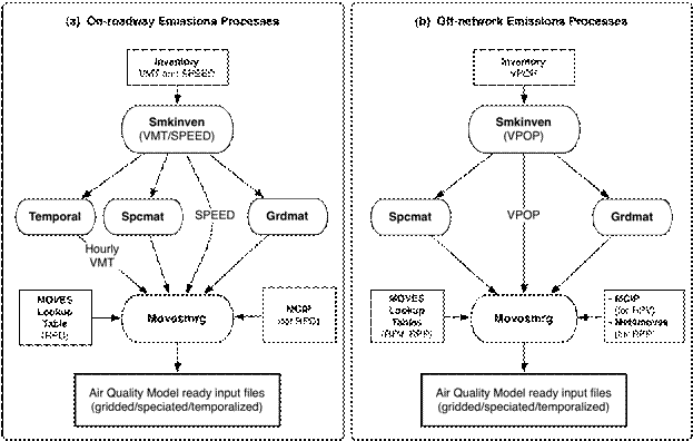
Figure
4. Flow diagrams of SMOKE-MOVES processing by emission processes.
The Rate Per
Distance (RPD) lookup table (see Table 22) is used to provide estimates of
on-roadway emissions processes from mobile sources, using a separate file for
each reference county. The on-road running processes that appear in this table
include running exhaust (EXR), crankcase running exhaust (CXR), brake wear
(BRK), tire wear (TIR), on-road evaporative permeation (EVP), on-road
evaporative fuel leaks (EFL), and on-road evaporative vapor venting (EFV). The
units of the emission rates in this table are grams/mile. The lookup fields for
the factors are temperature and average speed. There are 16 set speed bins
defined in Table 9 (i.e., avgSpeedBinID 1=2.5mph, 2=5mph, 3=10mph, …16=75mph).
The avgBinSpeed is used for interpolation in the RPD table.
4.2.2 Off-network Emissions Processes Emissions
Factors (RPV)
The Rate Per
Vehicle (RPV) lookup table (see Table 22) is used to provide estimates of
off-network emission processes (parked engine-off, engine starts, and idling),
except for the evaporative off-network vapor venting emissions process
(addressed in Section 4.2.3). A separate file is provided for each reference
county. The off-network emission processes include start exhaust (EXS),
crankcase start exhaust (CXS), off-network evaporative permeation (EVP),
off-network evaporative fuel leaks (EFL), extended idle exhaust (EXT), and
crankcase extended idle exhaust (CEI). Fuel month, temperature, and local
hourID are the lookup fields in this table, and hours are in the local time of
the countyID. The units of the emission rates are grams/vehicle/hour.
Note:
Although the units are grams/vehicle/hour, the number of vehicles (i.e.,
population) should not be temporally allocated to hours in SMOKE. Instead, a
county total of vehicle population should be multiplied by emission rates at
any given hour. The number of starts per vehicle by hour is already accounted
for in the MOVES lookup table.
4.2.3 Off-network Vapor Venting Emissions
Processes Emissions Factors (RPP)
The Rate Per
Profile (RPP) table (see Table 22) is used only to estimate emissions for
off-network fuel vapor venting (EFV) when the vehicle is parked. This process
type includes diurnal (when the vehicle is parked during the day) and hot soak
(immediately after a trip when the vehicle parks) emissions types. The process
depends on the rate of rise in temperature and the maximum temperature achieved
during the day for the diurnal emissions type, and on the hourly temperatures
for the hot soak emission type. The lookup fields for this table are fuel month
and hour of day. As with the RPV table, the units of the emission rates are
grams/vehicle/hour. The estimated emissions rates need to be multiplied by the
county vehicle population.
The reference
county lookup tables contain 24-hour emission rates per hour per vehicle using
a reference-county temperature profile with different minimum and maximum
temperatures. The average day county emissions are determined by interpolating
between the minimum and maximum temperatures for the county listed in the
Met4moves output file for SMOKE listed in Section 2.3.3.2. (Table 6).
Movesmrg is a new,
mobile-sources-only program, loosely based on the SMOKE program Smkmerge, that
combines the intermediate files produced by the other SMOKE programs (i.e.,
Grmdat, Spcmat, Temporal). Similar to Smkmerge, the main goal of Movesmrg is to
create (1) gridded, speciated, hourly air quality model-ready input files
and (2) county-level SCC summaries. The primary difference between Movesmrg and
Smkmerge is that Movesmrg uses the MOVES emission rate lookup tables to compute
emissions on the fly, by multiplying the emissions factors by hourly VMT (for
RPD) or by monthly or annual vehicle populations (for RPV or RPP).
Movesmrg must be run
three times to compute on-roadway and off-network (including vapor venting)
emissions processes individually, since the emission rate calculation methods
in SMOKE for these categories are quite different. Once all three emissions
processes have been computed, the emission output files can be merged
(optionally along with other 2‑D sectors separate from onroad) using
Mrggrid, which combines any number of 2‑D or 3‑D hourly, gridded,
and speciated emission data files. See the SMOKE user’s manual for more details
on the above programs.
4.3.1.1
Rate-Per-Distance (RPD) and Rate-Per-Vehicle
(RPV) Emission Calculations
For its RPD and RPV
(but not RPP) lookup table calculations, Movesmrg uses the gridded hourly
temperatures in GMT, and then adjusts the hour of the RPD and RPV lookup tables
from local time to GMT to get the emission rates for the reference county for
the appropriate month. The key lookup fields for the factors are hourly
temperature and average speed for the RPD lookup table calculation, and hourly
temperature and hour of the day in local time for the RPV table calculation.
4.3.1.2
Rate-Per-Profile (RPP) Emission Calculations
For its RPP (but
not RPD or PPV) lookup table calculations, Movesmrg uses the RPP lookup table
as an input file for the emission rates that depend not on the gridded hourly
temperatures, but on the temperature profiles output by the Met4moves program (Section
2.3.3.2). The emissions estimates based on the RPP table are computed for the
temporal averaging period specified for the temperature profiles, rather than
using hourly gridded meteorology.
4.3.1.3
List of Processing Pollutants Associated with
Processing IDs
Table 24 gives the
list of available MOVES pollutants and associates them with emissions processes
(i.e., processIDs or smokeProcIDs) from MOVES model, which were shown earlier
in Table 23. The information is used to create the MEPROC input file that
contains a list of MOVES emission processes and associated pollutants for
Spcmat.
For your information, on May 15, 2010, a
MOVES2010 Errata/Information sheet was prepared (http://www.epa.gov/otaq/models/moves/420b10026.pdf). It describes several issues with the
current version of MOVES. Two issues in particular (#12 and #14) could be very
important to some users:
·
Issue
#12: MOVES does not produce output for acrolein,
benzene, 1,3-butadiene, and formaldehyde for diesel vehicles if you request
processes other than the running exhaust process. This problem does not affect
gasoline vehicles.
·
Issue
#14: The extended idle process does not
produce records for benzene, formaldehyde, 1,3-butadiene, acetaldehyde, or acrolein
even though there are check boxes for these pollutants in the Pollutants and
Processes Panel.
Therefore, these toxics will not be
available for diesel vehicles in the MOVES driver script. All diesel vehicle
SCCs star with “2230”. See Appendix B
for more detail.
SMOKE must be run
after Met4moves and after MOVES. Once all output files from Met4moves and MOVES
processing scripts are ready, SMOKE programs Smkinven, Spcmat, Grdmat, and
optionally Temporal for the RPD mode must be run before Movesmrg runs
(Figure 4a and 4b).
Movesmrg
begins by reading environment variables and opening input files (these are
discussed in detail in Section 4.3.3). Environment variables include the source
category (which must be set to “M”) and flags that indicate the Movesmrg mode
to be run. Movesmrg can run in only one of three emissions processes (or modes)
at a time: (1) RPD, which calculates rate-per-distance emissions; (2) RPV, for
rate-per-vehicle emissions; or (3) RPP, for rate-per-profile emissions. Therefore, to process these three MOVES-based
lookup tables, SMOKE system including Movesmrg has to run three times.
Input files used by
Movesmrg include the grid description, processed inventory, and gridding and
speciation matrices. In RPD mode, output files from Temporal are opened so that
hourly VMT data can be read. While opening the input files, Movesmrg reads
inventory characteristics, including FIPS and SCC codes for each source. In
addition, Movesmrg checks for consistent grid information and a consistent
number of sources across the files. Movesmrg also opens several auxiliary
files, including the inventory data table file, the emission processes file (to
determine which emission processes and pollutants should be output), and
several cross-reference files relating to reference counties and other information.
Once the
environment variables and input files are checked/opened, Movesmrg performs
several setup steps, including reconciling pollutant and species names between
the MEPROC file, the INVTABLE file, and the speciation matrix (SMAT_L) from
Spcmat. Movesmrg also determines unit conversion factors for each output
species, and reads in county and state data corresponding to the FIPS codes in
the inventory.
Movesmrg uses the
gridding matrix (GMAT) to determine a list of grid cells associated with each source.
Because the gridding matrix is read into contiguous memory that mixes integer
and float storage, a special routine is used to split the gridding matrix into
separate arrays. These arrays are used during the main processing loop to
calculate the fraction of each source that should be allocated to the various
grid cells.
Movesmrg reads the
reference county information file (MCXREF) and builds data structures so that
it can easily access a list of sources for each reference county and can find
emission rates files for each reference county. Additionally, Movesmrg
determines the fuel month mapping used for each reference county based on the
fuel month input file (MFMREF).
After Movesmrg's
setup steps are complete, it opens the Movesmrg output files (MGTS_L or
MGSTS_S). Depending on the environment variable settings (described in Section
4.3.3.4), Movesmrg can output model-ready emissions (i.e., gridded, speciated,
hourly emissions) and/or state and county daily emissions totals for each
species.
Differences between RPD and RPV modes:
- RPD mode reads
average speed data from the inventory and hourly VMT data output from
Temporal
- RPV mode reads
VPOP data from the inventory
- RPD mode
processes pollutants and emission processes associated with VMT from the
MEPROC file
- RPV mode
processes pollutants and emission processes associated with VPOP
- RPD mode
interpolates the emission rates by speed bin and hourly temperature
- RPV mode
interpolates the emission rates by hourly temperature, using the local
hour
Differences between RPD/RPV and RPP modes:
- RPP mode uses
Met4moves output file (does not use hourly meteorological data as the RPD
and RPV modes do)
- RPP mode
interpolates the emission rates by temperature profile, instead of using hourly
temperature as the RPD and RPV modes do
4.3.3.1
MBINV: FF10 Activity Inventory Input File for
Smkinven
Smkinven requires
as input a new inventory file, MBINV. MBINV is an FF10 activity inventory
format for VMT, SPEED, and VPOP inventory data. The FF10 format is
list-directed and uses the header described in Table 25. Sample header records
are shown below:
#FORMAT=FF10_ACTIVITY
#COUNTRY US
#YEAR 2008
Table 25. FF10 format for MBINV
|
Line
|
Position
|
Name
|
Type
|
Required?
|
Description
|
|
+1
|
A
|
COUNTRY_CD
|
Char(2)
|
Y
|
Two-digit country code; default to
"US"
|
|
|
B
|
REGION_CD
|
Char(5)
|
Y
|
Five-digit FIPS code for state and
county
|
|
|
C
|
TRIBAL_CODE
|
Char(3)
|
N
|
Leave blank if not applicable
|
|
|
D
|
CENSUS_TRACT_CD
|
Char(20)
|
N
|
|
|
|
E
|
SHAPE_ID
|
Char(20)
|
N
|
|
|
|
F
|
SCC
|
Char(12)
|
Y
|
12-character SCC
|
|
|
G
|
ACT_PARM_TYPE_CD
|
Char(10)
|
N
|
|
|
|
H
|
ACT_PARM_UOFMSR
|
Char(20)
|
N
|
|
|
|
I
|
ACTIVITY_TYPE
|
Char(16)
|
Y
|
Activity variable names are VMT,
VPOP, and SPEED
|
|
|
J
|
ANN_PARM_VALUE
|
Real
|
Y
|
Activity values in unit of “miles/yr”
for annual VMT and “miles/hr” for SPEED
|
|
|
K
|
CALC_YEAR
|
Int
|
N
|
|
|
|
L
|
DATE_UPDATED
|
Char(8)
|
N
|
From LAST_UPDATED_DT, YYYYMMDD format
|
|
|
M
|
DATA_SET_ID
|
Int
|
N
|
|
|
|
N
|
JAN_VALUE
|
Real
|
N
|
Filled in only if data were provided
for January in unit of “miles/day” for monthly VMT. " if val < 1000,
write as #.####E##, else write as #.##
|
|
|
…
|
…
|
…
|
…
|
…
|
|
|
Y
|
DEC_VALUE
|
Real
|
N
|
Same as above
|
|
|
Z
|
COMMENT
|
Char
|
N
|
Comment
|
4.3.3.2
MEPROC: List of MOVES Emission Processes and
Associated Emission Pollutants for Spcmat
The MEPROC file, used by Spcmat, lists the emission processes and pollutants that will be generated by
MOVES for modeling on-road mobile sources. The format of the MEPROC file is shown in
Table 26. You can create your own MEPROC file using a master list of pollutants
associated with emission processes (Table 24).
Table 26. Format of MEPROC
|
Line
|
Position
|
Description
|
|
1+
|
A
|
Activity name (up to 16 characters)
|
|
|
B
|
Mobile emissions process (up
to 6 characters)
|
|
|
C+
|
Associated pollutant name(s)
for activity and process combination (Character)
|
Example of MEPROC for MOVES
VMT EXR CO
NOX TOG SO2 PM25OC PM25EC PM25SO4 NH3 BENZENE MTBE BUTADIE \
FORMALD ACETALD ACROLEIN
VPOP EXS CO
NOX TOG BENZENE MTBE BUTADIE FORMALD ACETALD ACROLEI
VMT EVP TOG
PM25OM PM10OM
VPOP EVP TOG
VMT EFL TOG
PM25OM PM10OM
VPOP EFL TOG
VMT EFV TOG
PM25OM PM10OM
VPOP EFV TOG
VMT CXR TOG
PM25OM PM10OM
VPOP CXS TOG
VPOP CEI TOG
VMT BRK PM25
BRAKE PM10BRAKE
VMT TIR PM25
TIRE PM10TIRE
4.3.3.3
Input/Output Files and Environment Variables for
Movesmrg
Figure 5 shows the
input and output files for the Movesmrg program. The inputs include the
country, state, and county codes file (COSTCY), the grid description file
(GRIDDESC), the inventory data table (INVTABLE), the reference county fuel
month file (MFMREF), the list of emission process and associated pollutants
file (MEPROC), the reference county cross-reference file (MCXREF) (Table 1),
the list of emission factors files by reference county file (MRCLIST, which is
discussed in more detail below Figure 5), the meteorology files (MET_CRO_2D),
the gridding matrix from Grdmat (MGMAT), the inventory file output from
Smkinven (MOBL), the speciation matrix from Spcmat (MSMAT), the Met4moves
output file for SMOKE (METMOVES), the MOVES-based lookup tables (RPD, RPV, and
RPP), and the daily hour VMT files from Temporal (MTMP_(day)). Note that
MET_CRO_2D, METMOVES, and MTMP_(day) are optional files that are included only
in certain situations, as shown in Figure 5.
Movesmrg outputs a
model-ready emissions file (MGTS_L or MGTS_S), a report file (REPMGTS_S), and a
log file (LOGFILE).
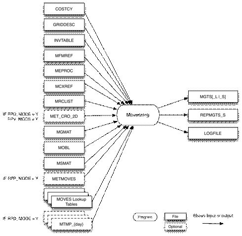
Figure
5. Movesmrg input and output files for mobile sources.
4.3.3.3.1 MRCLIST:
List of MOVES Lookup Tables for Movesmrg
The MRCLIST file is an input file for Movesmrg that contains the list of MOVES-based
lookup tables from the MOVES postprocessing script associated with reference
county and fuel month. The format of the MRCLIST file is shown in
Table 27. The user must define the location of the lookup tables using the
SMK_MVSPATH environment variable in order for Movesmrg to find these lookup
table files.
Table 27. Format of MRCLIST
|
Line
|
Position
|
Description
|
|
1+
|
A
|
Reference County (Integer)
|
|
|
B
|
Fuel Month (Integer)
|
|
|
C+
|
Associated MOVES-based lookup
table filename (Character)
|
Example of MRCLIST file for MOVES RPD
lookup tables
13121 4
rateperdistance_13121_apr.txt
13121 7
rateperdistance_13121_jul.txt
Example of MRCLIST file for MOVES RPV
lookup tables
13121 4
ratepervehicle_13121_apr.txt
13121 7
ratepervehicle_13121_jul.txt
Example of MRCLIST file for MOVES RPP
lookup tables
13121 4
rateperprofile_13121_apr.txt
13121 7
rateperprofile_13121_jul.txt
4.3.3.3.2 Input
Environment Variables for Movesmrg
The following
environment variables control the functioning of Movesmrg.
·
MRG_BYDAY: [default: blank]
String code that specifies which source
category is to use a by-day approach for the hourly input files. It must be set
to “M” for a Movesmrg run to create an output file for each day.
·
MRG_GRDOUT_YN: [default: N]
Determines whether Movesmrg produces a
gridded output file.
o Y: Read the gridding matrix produced by
the Grdmat program
o N: Do not read the gridding matrix
·
MRG_SPCOUT_YN: [default: N]
Determines whether Movesmrg produces a
speciated output file.
o Y: Read the speciation matrix produced by
the Spcmat program
o N: Do not read the speciation matrix
·
MRG_REPSTA_YN: [default: N]
Determines
whether Movesmrg produces a report of emission totals by state.
o Y: Produce the report
o N: Do not produce the report
·
MRG_REPCNY_YN: [default: N]
Determines whether
Movesmrg produces a report of emission totals by county.
o Y: Produce the report
o N: Do not produce the report
·
MRG_GRDOUT_UNIT: [default: file units]
String code that
permits user to change the unit of the gridded output file.
·
MRG_TOTOUT_UNIT: [default: file units]
String code that
permits user to change the unit of the state/county total report file.
·
RPD_MODE: [default: N]
Determines
whether Movesmrg processes rate-per-distance emissions.
o Y: Process rate-per-distance emissions
o N: Do not process rate-per-distance
emissions
·
RPV_MODE: [default: N]
Determines
whether Movesrg processes rate-per-vehicle emissions.
o Y: Process rate-per-vehicle emissions
o N: Do not process rate-per-vehicle
emissions
·
RPD_MODE: [default: N]
Determines
whether Movesmrg processes rate-per-profile emissions.
o Y: Process rate-per-profile emissions
o
N: Do
not process rate-per-profile emissions
·
SMK_EF_MODEL: [default: MOBILE6]
Name of the
emission rate model to use. To use the MOVES model, it must be set to “MOVES”.
·
SMK_MVSPATH: [default: blank]
Location of
MOVES-based emissions output files.
·
SMK_SOURCE: [default: blank]
Sets the types of source category. It must
be set to “M” for a Movesmrg run.
·
TVARNAME: [default: TEMP2]
Name of
temperature variable to read from the meteorology files
for a Movesmrg run.
Office of Transportation and Air Quality
(OTAQ), “Motor Vehicle Emission Simulator (MOVES) 2010: User Guide,”
EPA-420-B-09-041, U.S.
Environmental Protection Agency, Research Triangle Park, NC, December 2009.
Office of Transportation and Air Quality
(OTAQ), “Technical
Guidance on the Use of MOVES2010 for Emission Inventory Preparation in State
Implementation Plans and Transportation Conformity” EPA-420-B-10-023, U.S. Environmental Protection Agency, Research Triangle Park,
NC, April 2010.
Office of Research and Development (ORD),
“Meteorology-Chemistry Interface Preprocessor Release Notes,” U.S.
Environmental Protection Agency, Research Triangle Park, NC, October 2009.
Institute for the Environment (IE), “Sparse
Matrix Operator Kernel Emissions (SMOKE) version 2.6 User’s Manual,” University
of North Carolina, Chapel Hill, NC, 2009a.
Institute for the Environment (IE),
“Emissions Modeling Framework Surrogate Tool: User’s Guide,” University of
North Carolina, Chapel Hill, NC, 2009b.